Exotic Options - Computational Methods for Quantitative Finance - page 81

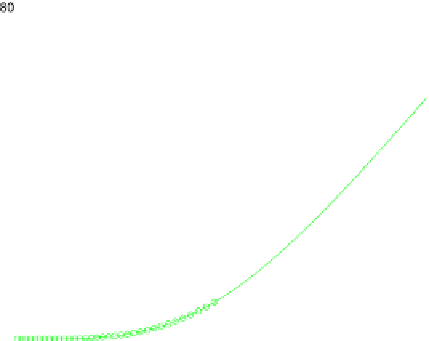
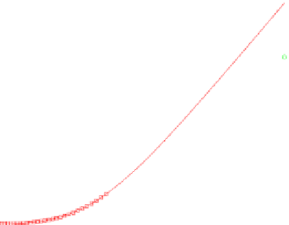
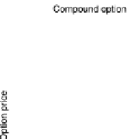
Fig. 6.3 Compound call and
underlying call option

We obtain the result by applying Theorem 4.3.1 to v R ,

| | ≤ | | + | |

v(t,x) − v R (t, x) v(t,x) − v R (t, x) v R (t, x) − v R (t, x)

≤ C 4 (T , σ ) e − γ 5 R + γ 6 | x | + C 3 (T , T 1 ,σ)e − γ 3 R + γ 4 | x | ,

where the option price v 1 satisfies (4.10) since g 1 satisfies (4.10).

Therefore, we have the weak formulation on the bounded domain G and in time-
to-maturity

Find u ∈ L 2 (( 0 ,T) ; H 0 (G)) ∩ H 1 (( 0 ,T) ; L 2 (G)) such that
(∂ t u, v) a BS (u, v) H 0 (G), a.e. in ( 0 ,T) + = 0 , ∀ v ∈

u( 0 ) = g(u 1 (T 1 − T )),

where the underlying option price u 1 satisfies

L 2 (( 0 ,T 1 − H 0 (G)) H 1 (( 0 ,T 1 − L 2 (G)) such that Find u 1 ∈ T) ; ∩ T) ;

a BS (u 1 ,v) H 0 (G), a.e. in ( 0 ,T 1 −

+ = ∀ ∈

(∂ t u 1 ,v) 0 , v T)

g 1 (e x ) u 1 ( 0 ) = | G .

Example 6.3.2 Consider a compound call option in a Black-Scholes market. Set
K 1 =

0 . 01. We plot the price of
the compound options and the corresponding underlying call price in Fig. 6.3 where
we used finite elements for the discretization. It can be seen that the price of the
compound option is lower than the price of the underlying option.

100, K = 20, T 1 = 1, T = 0 . 5, σ = 0 . 3 and r =