Lévy Models - Computational Methods for Quantitative Finance - page 139

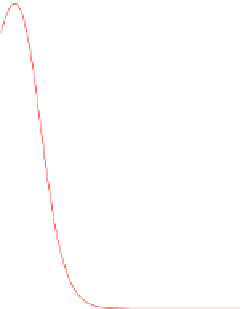
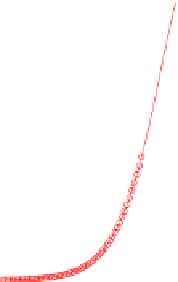
Fig. 10.1 Probability density
for the variance gamma
model ( top ) and the implied
volatility ( bottom )

than in the Black-Scholes case but is skewed as shown in Fig. 10.1 . For comparison,
we also plot the Gaussian density with the same variance. Additionally, we plot the
implied volatility of a European put option at S

100 for various strikes K . Here,
one nicely sees the so-called volatility smile. Note that in the Black-Scholes case
the implied volatility is constant.
For T

=

100, we compute the L ∞ -error at maturity t

= 1 and K = = T on the sub-

set G 0 =

= O

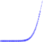
(N) and the Crank-
Nicolson scheme. It can be seen in Fig. 10.2 that for the finite element method we
again obtain the optimal convergence rate

(K/ 2 , 3 / 2 K) . We use constant time steps with M

(h 2 ) rather than

O O

(h) for the finite

difference method.