Overview and Fundamental Ideas - Wave Propagation in Drilling, Well Logging and Reservoir Applications - page 25

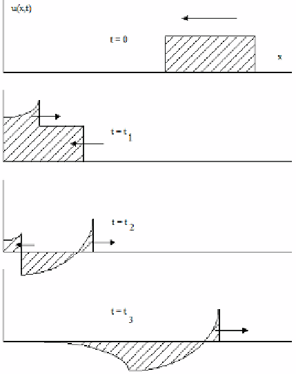
1.5.3.1 Example 1-10a. Rectangular pulse.
Figure 1.3b shows how a rectangular pulse is distorted at a pure elastic
boundary (with M = = 0); its closed form solution is given by Graff (1975).
We next determine the exact distortion effects for two important types of
incident waves.

1.5.3.2 Example 1-10b. Impulse response.
The time response of a system to an “impulse input” is important in
“control theory” because it contains all of the system' s dynamic characteristics,
e.g., reflections, attenuation and distortions. We consider an ideal impulse, that
is, an infinitely thin pulse of infinite height having bounded energy. This
incident pulse, heading toward the reflector at x = 0, is “set off” at t = 0; it is
described by an infinitesimally narrow “Dirac delta function” (t) discussed in
the next section. Following our recipes there, the use of Equation 1.63 leads to
the exact solution

u(x,t) = A {(t +x/c)/t ref } - A {(t -x/c)/t ref }
+ { 2 ATt ref /[ c(a-b)]}{ae a(ct-x) - be b(ct-x) } (1.64)

Figure 1.3b. Shape distortion due to elastic boundary.