Geology Reference
In-Depth Information
for example, represents a one-dimensional waveguide, but the term is generally
used to describe wave motions with one and two “cross-space” or “modal”
dimensions. Waves in waveguides are called “modal waves.”
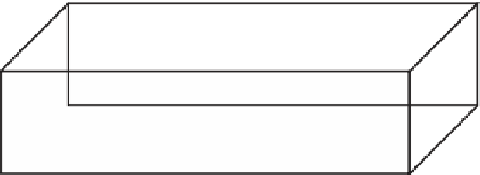
In anticipation of later work in MWD mud pulse telemetry, applicable also
to transient swab-surge in borehole annuli, we consider a model waveguide
problem for fluid flow acoustics. To keep the analysis simple, we study sound
propagation in the three-dimensional rectangular duct shown in Figure 3.2.
3D source and plane wave
Figure 3.2.
Simple rectangular waveguide.
Many excellent references to classical acoustics are available, e.g., Mason
(1942), Kinsler and Frey (1950), Morse and Ingard (1968) and Pierce (1981). In
this example, we hope to cover the fundamental ideas behind physical acoustics
and the mathematical techniques underlying waveguide analysis. In the simplest
case, the momentum laws governing fluid flow are the “Navier-Stokes
equations” for constant viscosity flow,
( u/ t + u u/ x + v u/ y + w u/ z) =
= - p/ x + (
2
u/ x
2
+
2
u/ y
2
+
2
u/ z
2
)
(3.16)
( v/ t + u v/ x + v v/ y + w v/ z) =
= - p/ y + (
2
v/ x
2
+
2
v/ y
2
+
2
v/ z
2
)
(3.17)
( w/ t + u w/ x + v w/ y + w w/ z) =
= - p/ z + (
2
w/ x
2
+
2
w/ y
2
+
2
w/ z
2
) (3.18)
Here u(x,y,z,t, v(x,y,z,t), and w(x,y,z,t) are “Eulerian velocities” at the fixed
point (x,y,z), in the directions of the x, y and z axes, respectively, and t is time.
Also, p(x,y,z,t) and (x,y,z,t) represent pressure and mass density per unit
volume. In transient compressible flows, density and velocity fields are coupled
by mass conservation,
/ t + ( u)/ x + ( v)/ y +
( w)/ z = 0
(3.19)
Despite the apparent generality of the above equations, the right sides in
Equations 3.16 to 3.18 apply to Newtonian flows only, that is, to fluids with
linear stress and strain rate relationships, and then, specifically to fluids having
constant viscosity. Note that drilling muds and cements, typically non-


Search WWH ::

Custom Search