Point Spread Function-Based Approaches to Three-Dimensional Scene Reconstruction - 3D Computer Vision: Efficient Methods and Applications - page 178

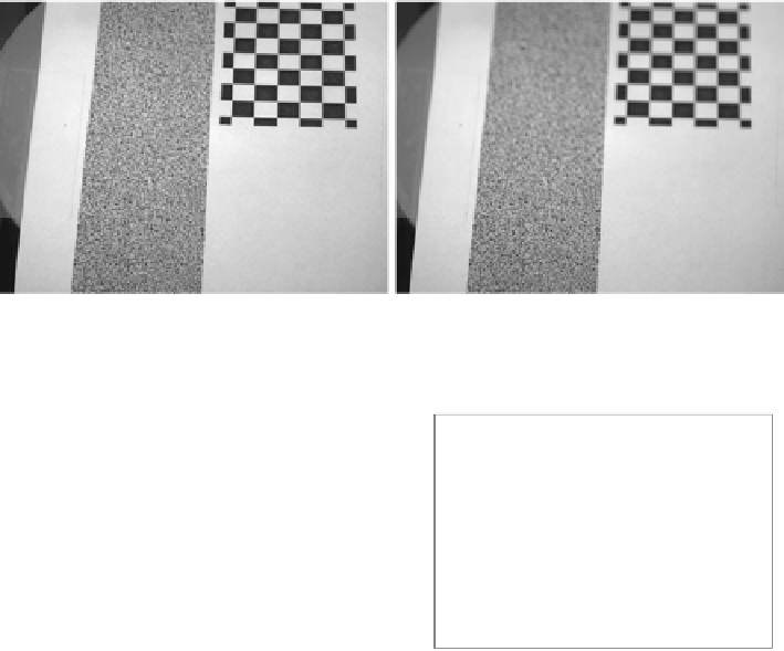
Fig. 4.9 Pixel-synchronous image pair ( left : κ = 8, right : κ = 2) used for calibration of the

depth-defocus function with a stationary camera

Fig. 4.10 Depth-defocus
function obtained with a
stationary camera based on
the calibration pattern shown
in Fig. 4.9

Moving Camera The description of the moving camera setting is adopted from
Kuhl et al. ( 2006 ). Calibrating the depth-defocus function

S

(z) for a given lens cor-
responds to determining the parameters φ 1 , φ 2 , φ 3 , and f in ( 4.15 ). This is achieved
by taking a large set of measured (σ, z) data points and performing a least-squares fit
to ( 4.15 ), where z is the distance from the camera and σ the radius of the Gaussian
PSF G σ used to blur the well-focused image according to
I ij = G σ ∗ I if i . (4.16)

Here, I if i represents a small region of interest (ROI) around feature i in image f i in
which this feature is best focused, and I ij an ROI of equal size around feature i in
image j .
For calibration, an image sequence is acquired while the camera approaches a
calibration rig displaying a chequerboard. The sharp black-and-white corners of the
chequerboard are robustly and precisely detectable with the method of Krüger et
al. ( 2004 ), even in defocused images. Small ROIs around each corner allow the
estimation of defocus using their grey value variance χ . The better focused the
corner, the higher the variance χ .
It was found experimentally that the parameterised defocus model according
to ( 4.15 ) is also a reasonable description of the dependence of χ on the depth z .