Graphics Reference
In-Depth Information
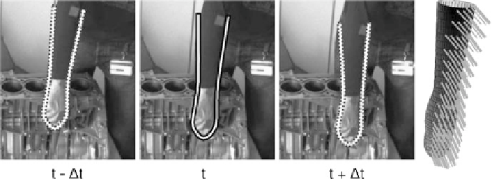
Fig. 2.11
Projected three-dimensional contour model for camera 1 at time steps
(t
−
t)
,
t
,and
(t
+
t)
.The
lines
indicate the amount and direction of motion for each point on the model surface
scene flow). At time step
t
the projected contour of the estimated three-dimensional
pose is shown as a solid curve, while the images at the time steps
(t
±
t)
depict
the projected contour of the pose derivative.
Step 2: Learn Local Probability Distributions from all
N
c
Images
For all
N
c
camera images
I
c
and for all
N
t
time steps, compute the local probability dis-
tributions
S
c,t
(
m
T
,Σ
T
)
on both sides of the projected three-dimensional contour
model, defined by camera
c
and time step
t
. This step is similar to step 1 of the CCD
algorithm, the only difference is that the probability distributions
S
c,t
(
m
T
,Σ
T
)
on
both sides of the curve are learned for all
N
c
cameras images
I
c,t
at all
N
t
time
steps.
Step 3: Refine the Estimate (MAP Estimation)
The curve density parameters
(
m
T
,Σ
T
)
are refined towards the maximum of (
2.31
) by performing a single step
of a Newton-Raphson optimisation procedure. The learned spatio-temporal proba-
bility distributions
S
c,t
(
m
T
,Σ
T
)
are used to maximise the joint probability
S
c,t
(
m
T
,Σ
T
)
p
T
I
c,t
}
=
p
I
c,t
|
m
T
, Σ
T
)
|
|{
·
p(
T
(2.31)
c
t
with
S
c,t
(
m
T
,Σ
T
)
representing the probability distributions of the pixel grey values
close to the projected curve in image
I
c,t
(camera
c
, time step
t
). The underlying
assumption is that the images are independent random variables. As in the original
CCD framework, a numerically favourable form of (
2.31
) is obtained by computing
the log-likelihood. The SF algorithm can be interpreted as a top-down, model-based
spatio-temporal three-dimensional pose estimation approach which determines a
three-dimensional pose and its temporal derivative. The advantage is that tempo-
ral and spatial constraints are handled directly in the optimisation procedure.
Search WWH ::

Custom Search