Biomedical Engineering Reference
In-Depth Information
1.0
1.0
(a)
m
<1
(b)
m
=1
0.8
0.8
m
= 0.5
0.6
0.6
0.4
0.4
0.2
0.2
0.0
0
0.0
2
4
6
8
10
0
2
4
6
8
10
σ
σ
1.0
(c)
m
>1
m
= 6
0.8
m
= 3
0.6
m
= 2
0.4
0.2
0.0
0
2
4
6
8
10
σ
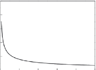
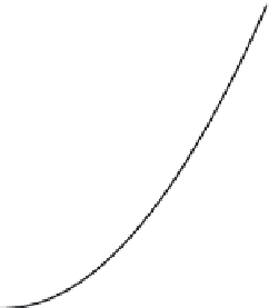
FIGURE 6.32
Three failure modes of materials (other parameters are
η
= 5,
σ
o
= 0): (a) decreasing failure rate (DFR) of an early
failure with
m
< 1; (b) constant failure rate (CFR) of random failure with
m
= 1; and (c) increasing failure rate
(IFR) of a wearout failure with
m
> 1.
• A value of
m
> 1 indicates that the system belongs to a wearout failure model
and the failure rate increases with time (IFR). In addition, the slope of failure
rate function curve increased with increasing the Weibull modulus, as shown in
Figure 6.32c. This situation occurs if there is an aging process, or parts that are
more likely to fail as time go on.
The characteristic strength
σ
c
corresponds to the strength at which the cumulative fail-
ure probability is 63.2%. The minimum strength
σ
o
means that the failure probability of
HACs lower than this strength is zero. The Weibull model is a very flexible life distribution
model with two defining parameters, which are the Weibull modulus (
m
) and the charac-
and the charac-
teristic strength (
σ
c
).
The cumulative failure probability
F
(
σ
i
) is estimated using the Benard's median rank in
Equation 6.35 [249], which is a very close approximated solution of a statistical function
[248,250], and the reliability function
R
(
σ
i
) with a relation of
R
(
σ
i
) = 1 −
F
(
σ
i
) is defined as the
survival probability [239]. Through the natural logarithmic (ln) graphs for the cumulative
failure probability at each corresponding bonding strength
σ
i
(
i
= 1-20) of the specimens, it
can graphically evaluate the Weibull modulus (
m
) from the slope of a least-squares fitting
method of Equation 6.36.

Search WWH ::

Custom Search