Sustainability and Stability - Bioprocess Engineering: Kinetics, Biosystems, Sustainability and Reactor Design - page 798

which can be reduced to a quadratic equation:

1 m max
Dþ k d

SþS 2

K S þ = K I ¼ 0 (E16-2.12)

Two roots can be obtained from Eqn (E16-2.12) :

s

K I
4

m max

Dþ k d 1

m max

Dþ k d 1 2

K I
2

S ¼ K S K I (E16-2.13)

To determine the value of biomass concentration, we substitute Eqn (16-2.9) into (E16-2.5a) to
yield

YF X = S D
Dþk d ðS 0 SÞ

X ¼ (E16-2.14)

Therefore, we have obtained three solutions:

(1) X ¼ 0, S ¼ S 0 ¼ 100 g/L;
(2) S ¼ 2.1922 g/L, X ¼ 62.597 g-X/L; and
(3) S ¼ 22.8077 g/L, X ¼ 49.403 g-X/L.

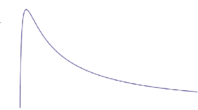
Fig. E16-2.2 shows an illustration of the steady-state solutions. There are two intercepts of
the specific mass removal rate line with the specific mass growth rate curve for S S 0 . There-

fore, both intercepts are steady-state solutions; their corresponding substrate concentration
values are given above.
(b) Steady states 1) and 2) can be operated on as they are stable steady states. One can
imagine steady state 1) being stable as when cells are washed out and not introduced

<

0.07

0.06

SMR X = D + k d

0.05

0.04

SMG X = µ G

0.03

0.02

0.01

0.00

0 50 100 150 200

S, g/L

FIGURE E16-2.2 Graphic interpretation of the steady-state solution.