Geoscience Reference
In-Depth Information
a
b
population density
house density
< 1,000
< 100
100 - 500
500 - 1,000
1,000 - 2,000
2,000 - 5,000
5,000 - 10,000
10,000 - 20,000
1,000 - 2,000
2,000 - 5,000
5,000 - 10,000
10,000 - 20,000
20,000 - 50,000
50,000 - 100,000
> 100,000
> 20,000
c
d
road density
distance to highway
<5%
5-10%
> 1.6 KM
0.0 - 0.2 KM
45-50%
51-60%
61-65%
11-15%
0.2 - 0.4 KM
16-20%
20-25%
25-30%
30-35%
35-45%
0.4 - 0.6 KM
66-70%
0.6 - 0.8 Km
71-75%
0.8 - 1.0 KM
76-80%
>80%
1.0 - 1.2 KM
1.2 - 1.6 KM
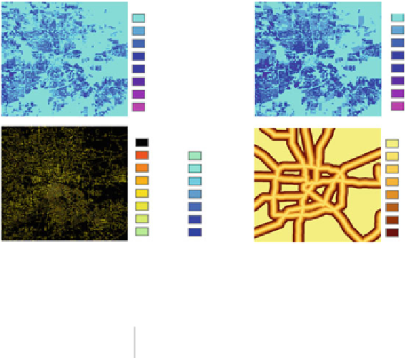
Fig. 12.3
The visualization of the socioeconomic value in Houston (
a
) Population density; (
b
)
House density; (
c
) Road density; and (
d
) Distance to highway
Table 12.3
The weight of socioeconomic indices
Population
density
Road
density
Distance
to highway
House
density
Houston
Barren/soil
3.67
3.50
3.40
4.00
Industrial/commercial
8.80
8.17
8.42
7.33
Grassland
3.18
2.75
3.36
4.90
Residential
9.46
8.08
6.25
8.92
Transportation
7.66
9.00
8.95
6.82
Woodland
2.82
2.58
3.18
4.70
A critical issue in the CA model is the provision of proper methods to calibrate
the CA model to find appropriate coefficients for the diffusion factor, Markov
transition rules, and socioeconomic status (Hagen-Zanker and Lajoie
2008
;Van
Vliet et al.
2011
). To calibrate the model, we used the classified Landsat TM image
as empirical maps on the following dates: November 5, 1984; July 20, 1990; October
6, 1999; and November 9, 2000. We randomly selected an encoded weight number
(ranging from 1 to 10) for each factors, run the CA model using these weight
number, and compared the cells simulated in the CA model with the cells located
in the empirical maps to choose the weight number with the highest fitness. The
CA model was run at yearly intervals to represent one combination until the next
calibration year. These steps were repeated until the year of the last calibration map.
For the validation, the model's simulation output was compared to the empirical
map, occurring in the same simulated year (Pontius et al.
2004
; Pontius and Cheuk
2006
) through visual inspection and quantitative evaluation. In this research, we
adopted the classified map in October 31, 2011, as an empirical map and overlaid
it with the predicted map to generate a black-and-white error image. Meanwhile, an
error matrix was built up with the user's and producer's accuracy for each class as
well as the overall accuracy and Kappa for the entire landscape.


Search WWH ::

Custom Search