Geography Reference
In-Depth Information
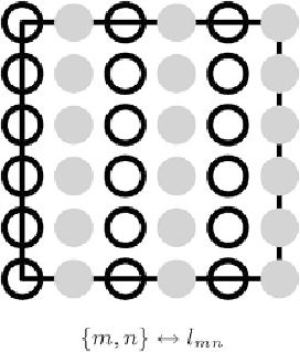
Fig. 21.8.
Polynomial diagram, the polynomial representation of longitude increments
l
−
l
0
, conformal coordi-
nates
of type Gauss-Krueger or UTM, the
solid dots
illustrate non-zero monomials, the
open circles
zero
monomials, according to
Cox et al.
(
1996
, pp. 433-443)
{
x, y
}
21-413 The Third Step: Global Conformal Coordinates in a Local Datum
By means of the bivariate series (
21.70
)ofBox
21.14
subject to the coecients of Boxes
21.20
and
21.21
, we have succeeded to express global conformal coordinates of type Gauss-Krueger
or UTM in terms of local ellipsoidal coordinates, namely the eastern coordinate
X
(
l
−
l
0
,b
−
b
0
,ρ,t
x
,t
y
,t
z
,α,β,γ,s,δE
2
) and the northern coordinate
Y
(
l
b
0
,ρ,t
x
,t
y
,f
z
,α,β,γ,s,δE
2
).
Only the transformation (the third step) from local ellipsoidal coordinates
{l − l
0
,b− b
0
}
is left.
Such a transformation is achieved by a bivariate series inversion outlined in
Grafarend
(
1996
),
namely of type (
21.66
). In Box
21.14
, we have reviewed the result of a bivariate series inversion
of conformal type subject to the coecients given by Boxes
21.23
and
21.24
as well as illustrated
by Figs.
21.8
and
21.9
.
−
t
0
,b
−
Box 21.22 (Series inversion of a local system of conformal coordinates of type Gauss-Krueger
or UTM into ellipsoidal coordinates).
l − l
0
=
y
ρ
−
y
00
+
l
30
x
ρ
3
y
p
−
y
00
2
=
l
10
x
ρ
+
l
11
x
+
l
12
x
ρ
+O(4)
,
p
b
−
b
0
=
(21.79)
=
b
01
y
ρ
− y
00
+
b
20
x
2
+
b
02
y
ρ
− y
00
2
+
b
21
x
ρ
2
y
ρ
− y
00
ρ
+
b
03
y
y
00
3
ρ
−
+O(4)
.


Search WWH ::

Custom Search