Geography Reference
In-Depth Information
S
2
R
+
P
2
O
E
λ
1
,λ
2
, right eigenvectors
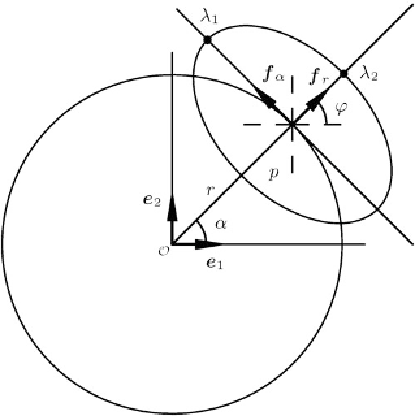
Fig. 1.11.
Orthogonal projection
onto
, polar coordinates, right Tissot ellipse
{
f
α
,
f
r
|
p
}
, right eigenvalues
{
λ
1
,λ
2
}
, image of parallel circle
Solution (the first problem).
By means of detailed derivations given in Boxes
1.13
and
1.14
, we aim at an analytical analysis of
the right Cauchy-Green deformation tensor in Cartesian coordinates
{x, y}
and in polar coordi-
nates
{α,r}
, which cover the projection plane
P
. The right mapping equations
{Λ
(
x, y
)
,Φ
(
x, y
)
}
and
{Λ
(
α
)
,Φ
(
r
)
}
are given first. They are constituted from the identities
x
=
X
=
R
cos
Φ
cos
Λ
and
y
=
Y
=
R
cos
Φ
sin
Λ
,where
{Λ, Φ}
are the spherical coordinates.
{Λ, Φ}
or
{
longitude,
latitude
}
label a point in
S
2
O
+
,
which are points in the northern hemisphere. Second, we compute the right Jacobi matrices J
r
(
x, y
)
and J
r
(
α, r
) in Cartesian coordinates
2
R
+
. We use the symbol + in order to allow only positive values
Z ∈
R
. While J
r
(
x, y
)isa
fully occupied matrix, J
r
(
α, r
) is diagonal. Third, this difference continues when we are going to
compute the right Cauchy-Green matrices C
r
(
x, y
)andC
r
(
α,r
). Again, C
r
(
x, y
) is a fully occu-
pied symmetric matrix, while C
r
(
α,r
) is diagonal. Fourth, in Box
1.13
, we represent the right
Cauchy-Green deformation tensor as a tensor of second order in the Cartesian two-basis
e
μ
⊗
{
x, y
}
and in polar coordinates
{
α, r
}
e
ν
2
=span
for all
{
μ, ν
}
=
{
1
,
2
}
.Notethat
R
{
e
1
,e
2
}
,where
{
e
1
,e
2
|O}
is an orthonormal two-leg
at
e
2
.Incon-
trast, the algebra of the right Cauchy-Green deformation tensor in Box
1.14
, represented in polar
coordinates, is slightly more complicated. A placement vector
x
(
α,r
)
O
.Remarkably,C
r
(
x, y
) includes the components
e
1
⊗
e
2
,e
1
⊗
e
2
+
e
2
⊗
e
1
,and
e
2
⊗
2
O
∈
P
is locally described
r
spanned by the tangent vectors
g
1
=
D
α
x
and
g
1
=
D
r
x
. In polar
by the tangent space
T
x
M
, the matrix of the right metric is given by G
r
=diag(
r
2
,
1), a diagonal matrix.
The first differential invariant of
coordinates
{
α,r
}
r
2
O
is given by (d
s
)
2
=
f
(d
α,
d
r
). The basis
g
1
,
g
2
M
∼
P
{
}
,
, also called
co-frame
, is computed next, namely by G
−
1
(
α, r
). Due to the
orthogonality of the two-leg
{
g
1
,
g
2
|p}
, the co-frame amounts to
g
1
=
g
1
/
g
11
and
g
2
=
g
2
/g
22
,
respectively. Question: “Why did we bother you with the notation of the co-frame
{
g
1
,
g
2
|p}
?”
Answer: “Often the moving frame
{
g
1
(
α, r
)
,
g
2
(
α, r
)
}
is called
covariant
, accordingly its dual
which is
dual
to
{
g
1
,
g
2
}


Search WWH ::

Custom Search