Geography Reference
In-Depth Information
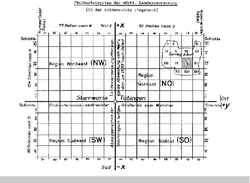
Fig. 20.6.
An example of a Soldner map, centered at the Tubingen Observatory, Germany, original map.
x
≡
y
c
,
y
≡
y
c
20-32 Second Problem of Soldner Coordinates: Geodetic Parallel
Coordinates, Input
{L, B, L
0
,B
0
}
Versus Output
{x
=
y
c
,y
=
x
c
}
The inverse problem to derive the Soldner coordinates
{
x
=
y
c
,y
=
x
c
}
from the given values
of
is again solved by series inversion, the result of which is provided by (
20.127
)
and (
20.128
), with (
μν
)
x
and (
μν
)
y
as Soldner inverse series coecients (Figs.
20.5
and
20.6
).
{
L, B, L
0
,B
0
}
∞
∞
(
μν
)
x
(
B
B
0
)
μ
(
L
L
0
)
ν
,
x
=
−
−
(20.127)
μ
=0
ν
=0
∞
∞
(
μν
)
y
(
B
B
0
)
μ
(
L
L
0
)
ν
.
y
=
−
−
(20.128)
μ
=0
ν−
0


Search WWH ::

Custom Search