Geography Reference
In-Depth Information
S
2
R
onto the tangent space
T
N
S
2
R
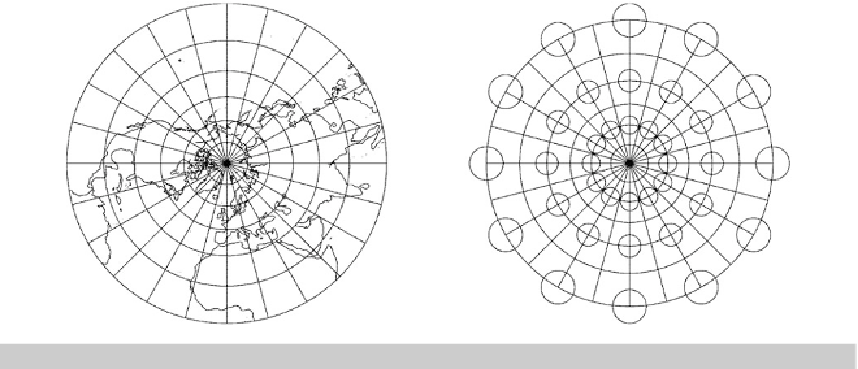
, Tissot ellipses, polar aspect,
Fig. 5.7.
Conformal map (UPS) of the sphere
graticule 15
◦
, shorelines
5-23 Equiareal Mapping (Lambert Projection)
Let us postulate an
equiareal mapping
by means of the canonical measure of areomorphism, i.e.
Λ
1
Λ
2
= 1. Such an equiareal mapping of the sphere to the tangential plane of the North Pole is
illustrated by means of Fig.
5.8
that follows after Box
5.6
.
Question: “How can we construct the equiareal mapping
equations” Answer: “Following the procedure of Box
5.6
,we
here depart from the general representation of
Λ
1
and
Λ
2
.
The postulate of an equiareal mapping leads us to the char-
acteristic differential equation, which we solve by separa-
tion of variables. We use the initial condition
r
(0)=
f
(0)=2
R
sin
Δ
/2, namely the polar coordinate
r
as a function of the
colatitude
Δ
, also called
polar distance
.Thepolarcoor-
dinate
α
=
Λ
is fixed by the postulate of an azimuthal
projection. The parameterized equiareal mapping is finally
used to compute the left principal stretches, namely
Λ
1
=
1
/
cos
Δ/
2
,Λ
2
=cos
Δ/
2. They build up the left eigen-
vectors along the East unit vector
E
Λ
and the North unit
vector
E
Φ
(the South unit vector is
E
Δ
=
−
E
Φ
). These
unit vectors are defined by
E
Λ
:=
D
Λ
X
/
and
E
Φ
:=
D
Φ
X
/D
Φ
X
. In addition, we have computed the
left maximal angular shear as well as the parameterized
inverse mapping
{Λ
(
x, y
)
,Φ
(
x, y
)
}
”.
D
Λ
X
The basic results of the equiareal azimuthal projection of the sphere to the tangential plane at
the North Pole are collected in Lemma
5.3
.

Search WWH ::

Custom Search