Biomedical Engineering Reference
In-Depth Information
10 nm
500 nm
μ Δ
z
IDFT
1
0.9
0.8
0.7
0.6
0.5
0.4
x
-
y
localization
σ
z
<
10 nm
σ
x,y
<
10 nm
0.3
0.2
0.1
0
640
z
localization
660
680 700 720
wavelength (nm)
740
760
780
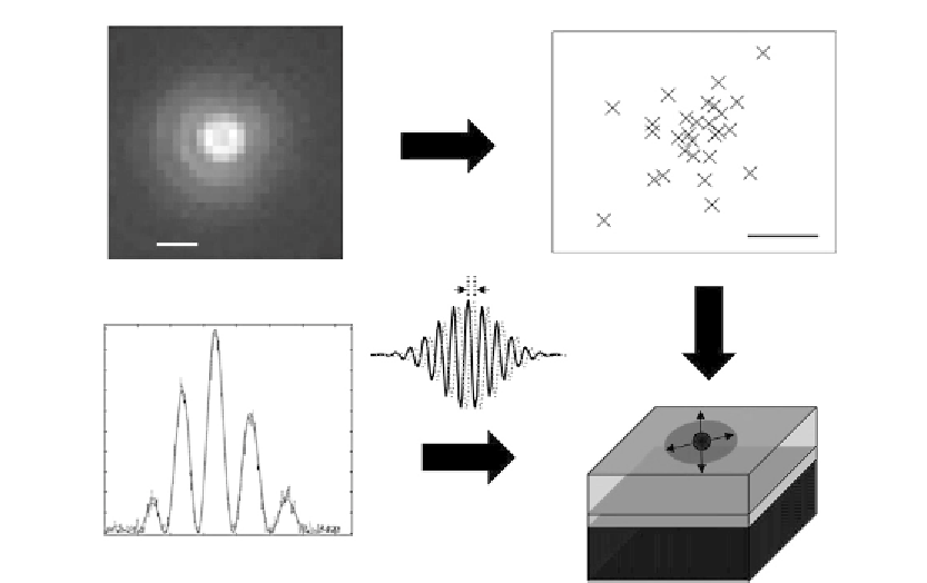
Figure 18.5
3D localization of a single fluorescent QD. A typical fluorescence image of a single QD is shown
in the top-left panel. Repetitive lateral localizations of the single QD are retrieved by analyzing the
recorded PSF as depicted in the top-right panel. Typical measured (dashed line) and fitted (solid
line) spectra of an individual QD are presented in the bottom-right panel. The axial localization of
the QD is obtained by Fourier analysis of the fitted spectra. As a result, an individual QD can be
localized in all three dimensions with a precision below 10 nm as illustrated in the bottom-right
panel. Source: This figure is partially reproduced from figures 2(a) and 3(a) of Ref.
[42]
with permission of
the Optical Society of America.
sample (
Figure 18.6A
) by the SD-FPM of
Figure 18.3A [41]
. To reduce the noise floor
fluctuations, these measurements were performed by averaging several consecutive images.
The two layers can be clearly observed over a wide transverse field (
.
1 mm). The mean
distance between the layers was measured to be 120.1
μ
m and closely matched the
calibrated 120
m separation of the layers. Importantly, the acquisition of the tomogram by
the SD-FPM system was performed without any scanning of the sample or focus—a key
advantage of SD-FPM which does not require any moving components to resolve axial
(depth) information. We carried out similar measurements by using the wide-field TD-FPM
setup of
Figure 18.2
and reconstructed a 3D image of the sample as presented in
Figure 18.6B
. We note that in contrast to SD-FPM the wide-field TD-FPM system requires
axial scanning of the sample to detect axial (depth) information; yet, no transversal
scanning is needed to reconstruct a 3D image of the specimen.
μ
Search WWH ::

Custom Search