Biomedical Engineering Reference
In-Depth Information
rad
1
0.5
0
6
800
5
800
700
700
4
600
600
500
500
3
400
400
2
800
300
700
800
600
300
700
200
500
600
1
400
500
200
300
100
400
200
(B)
(A)
0
100
300
0
100
0
200
100
0
0
rad
rad
1.6
1.4
2
800
800
700
700
1.2
1.5
600
600
1
500
0.8
0.6
0.4
0.2
0
500
1
400
400
800
800
0.5
300
300
200
700
700
600
600
200
500
500
400
400
0
300
300
100
100
(C)
(D)
200
200
100
100
0
0
0
0
0
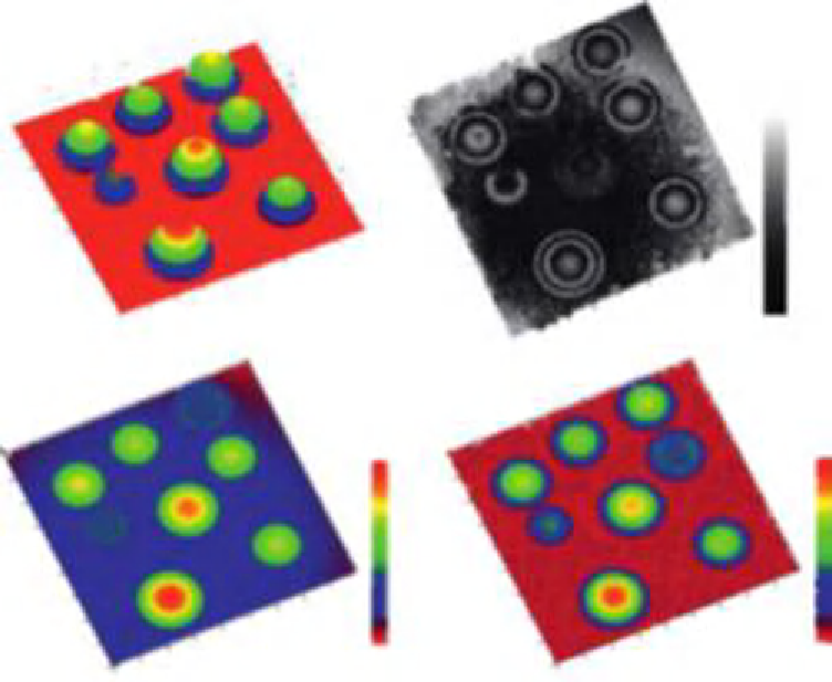
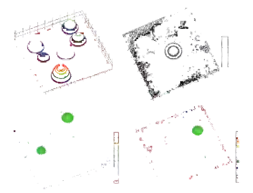
Figure 7.5
Background removal for simulated cells. (A) Simulated cells on the flat substrate, (B) single
wavelength (635 nm) simulated phase images with added phase, (C) dual-wavelength unwrapped
phase image, and (D) dual-wavelength unwrapped phase image with background removed.
first iteration (dotted line), while removing the original peaks, also “dives” under the
original curved profile near the ends of the frame. As a result (dashed line), the curvature is
overcompensated. However, it can be fixed by modifying the algorithm's step 2 in the
following way:
2a. Compare the polynomial surface with the original image.
2b. Find the maximum difference between the fit and the original profiles.
2c. Add a fraction of that maximum difference to the polynomial surface.
This modification, although making the convergence much slower, does result in a flat
background (see
Figure 7.6
—solid line). The fraction, used in step 2c can be as high as
95% and is limited only by computational rounding error as well as the computational
speed (the higher is the number, the longer it takes for the method to converge). The result
Search WWH ::

Custom Search