Image Processing Reference
In-Depth Information
(
a
)
(
b
)
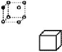
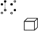
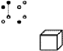
Fig. 4.8.
Local patterns in the 6-neighborhood and
2
×
2
×
2
local areas: (
a
)Local
patterns in the 6-neighborhood. (Total is
20
cases. Figures show only the cases in
which the center is a 0-voxel. Patterns symmetric to these are neglected.); (
b
)All
2
×
2
×
2
local patterns.
ing to individual local pattern of an input image. The minimum size of a local
area is
2
3
voxels.
There are
2
8
=
256
different binary patterns and
2
27
=
134
,
217
,
728
patterns for these local areas, respectively. This means
2
a
local functions are
possible, where
a
=
2
8
×
2
×
2
voxels and the second smallest is
3
×
3
×
and
2
27
×
×
×
×
3
neighborhoods,
respectively. They will be too large to be treated by a simple exhaustive
enumeration or by other intuitive methods. To understand features of each
3
for
2
2
2
and
3
3
3
pattern is not easy work even for the human visual system. Thus
suitable quantitative features characterizing individual patterns or a subclass
of patterns are strongly desired. The connectivity index and the connectivity
number introduced in the previous section are such examples.
×
3
×
4.5.1
2
×
2
×
2
local patterns
All
2
2
local patterns are enumerated without much diculty. In, fact,
only
22
cases exist after excluding rotation symmetry pairs and line symmetry
pairs. All of these
22
cases are shown in Fig. 4.8.
×
2
×
Remark 4.13.
Let us present three examples of applications of
2
×
2
×
2
patterns.
(a) Calculation of the Euler number: The Euler number of a 3D figure is cal-
culated by enumerating
2
×
2
×
2
patterns. Details are presented in Sec-
tion 4.7.


Search WWH ::

Custom Search