Information Technology Reference
In-Depth Information
Plot of ROC Curves
1
Plot of ROC Curves
AT−1
AT−2
AT−3
a
b
c
1
AT−1
AT−2
AT−3
a
b
c
convex hull
0.9
0.9
0.8
0.8
0.7
0.7
0.6
0.6
0.5
0.5
0.4
0.4
0.3
0.3
0.2
0.2
0.1
0.1
0
0
0
0.1
0.2
0.3
0.4
0.5
0.6
0.7
0.8
0.9
1
0
0.1
0.2
0.3
0.4
0.5
0.6
0.7
0.8
0.9
1
false positive fraction
false positive fraction
(a)
(b)
S2
Plot of ROC Curves
1
AT−1
AT−2
AT−3
a
b
c
convex hull
S1
0.9
0.8
0.7
0.6
0.5
0.4
0.3
0.2
0.1
0
0
0.1
0.2
0.3
0.4
0.5
0.6
0.7
0.8
0.9
1
false positive fraction
(c)
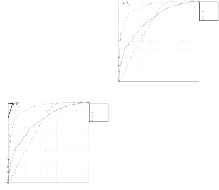
Fig. 2.
(a) 3 ROC points and 3 ROC curves representing 6 AT systems. (b) Their ROC
Convex Hull. (c) 2 iso-performance lines for 2 different sets of conditions
computational geometry and decision analysis. Thus, once the ROC points or
ROC curves have been computed for the different participants we proceed as
follows to select the best AT systems. Firstly, we compute the convex hull of the
set of ROC points that symbolizes a composite AT system. Secondly, we compute
the set of iso-performance lines corresponding to all possible cost distributions.
Finally, for each iso-performance line we select the point of the ROCCH with
the largest TPF that intersects it. Figure 2 (a) depicts the AT systems analyzed
above. To select which systems will be of interest for a collection of unknown
conditions we compute the convex hull such as it is shown in Fig. 2 (b) where the
circled points denote the points that forms part of the ROCCH and therefore can
be optimal for a number of conditions. Thus they form part of the composite
AT system chosen as a winner. Finally, Fig. 2 (c) shows two illustrative iso-
performance lines corresponding to the slopes
S
2
. Thus, for each of the
different sets of conditions that determine the values of slopes
S
1
and
S
1
and
S
2
the AT
systems
a
and
b
will be the optimal respectively.