Information Technology Reference
In-Depth Information
correlation and equalize the energy distribution, and then undergo a second layer of
orthogonal transformation such as DFT. QIM is carried out in the dual-transform
domain. The marked image is obtained by a reverses sequence of operations: IDFT,
de-scrambling, replacement of the chosen DCT coefficients with modified ones and
finally, block-IDCT.
3
Statistical Properties of DCT Coefficients
Based on the central limit theorem, it has been conjectured that the AC coefficients of
DCT obey a Gaussian distribution [6]. Other authors suggest different probability
density functions such as Laplacian [7] and generalized Gaussian [8]. The PDF of
zero-mean generalized Gaussian distribution is:
−
ν
v
α
(
ν
)
x
()
f
x
=
exp
α
(
ν
)
,
(2)
()
2
δ
Γ
1
ν
δ
where α(ν) is defined as
()
()
Γ
3
/
v
()
α
v
=
.
(3)
Γ
1
/
v
In the above expressions, Γ(
.
) is a gamma function. The variablesν and δ are posi-
tive constants depending on the frequency index of the coefficients under considera-
tion.
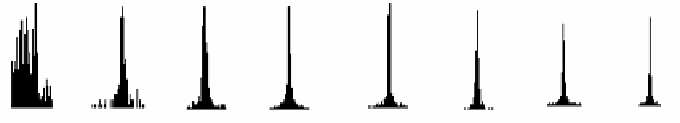
Fig. 2.
Histograms of DCT coefficients of different frequency components
Fig. 2 shows the histograms of the corresponding DCT coefficients in some blocks
of a test image Lena. Each block is sized 8×8. The first block corresponds to the DC
component, while the rest are AC components with different spatial frequencies (only
seven AC components are shown in the figure). Scaling of the histograms is kept
constant except for the DC component. It is observed that the distributions of all AC
components are approximately Gaussian. The variance of each histogram decreases
with increasing spatial frequency because energy in most natural images is generally
concentrated in low frequency bands. As can be seen in the figure, another feature is
that the lines are distributed compactly and roughly symmetrical about the mean
without obvious missing segments. In the rest of the paper, only AC components are
considered.