Information Technology Reference
In-Depth Information
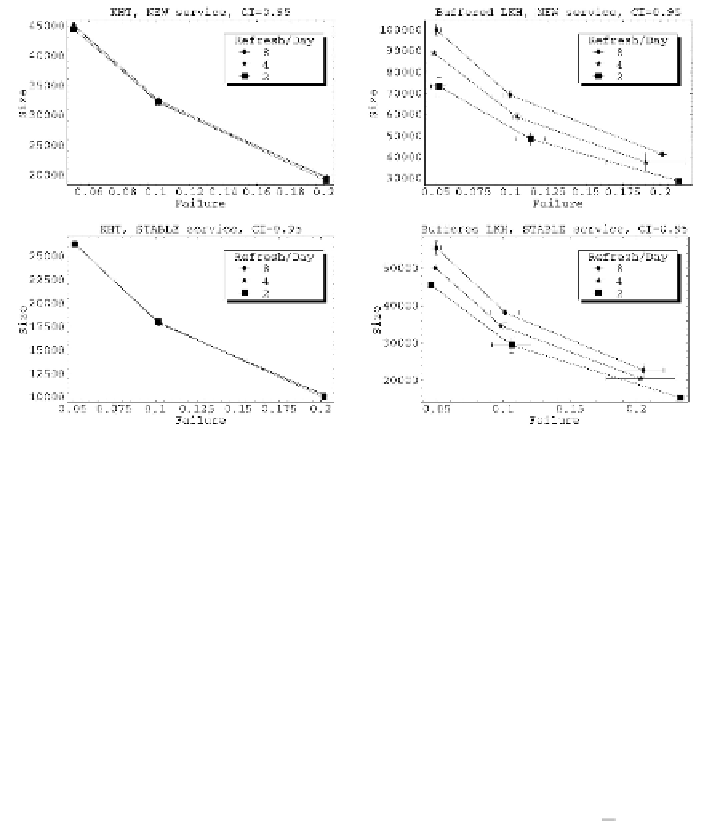
Fig. 6.
Comparing KHT with buffered LKH
p
fail
, the probability of
failing to decrypt the content by a valid client while accessing the service. As
we recall from Section 3, this is a side effect of mis-predicting the KHT-WS. In
the case of KHT we dynamically change the size of the KHT cache to keep that
probability to a certain constant target. As we can see from the tight confidence
intervals in Fig. 6 a) and Fig. 6 c) this is very effective in practice. However, in
the case of Buffered LKH, the only mechanism that we have to decrease
The horizontal axis of the graphs in Fig. 6 show
p
fail
is
to accumulate key updates from several refresh periods, and even though we also
dynamically adjust the number of refresh periods aggregated, this adjustment
has larger granularity. This is reflected in Fig. 6b) and Fig. 6d) that show larger
p
fail
confidence intervals.
The vertical axis of the graphs in Fig. 6 reflects the average size
,innumber
of elementary key update entries, of the annotation added to the content by
the CDBE. This average is computed per access, so that multiplied by the total
number of accesses we obtain the “wasted bandwidth” tha
t
the scheme to recover
off-line members requires. Again, confidence intervals for
S
S
in the Buffered LKH
are greater than in KHT for similar reasons.
Graphs in Fig. 6 clearly show that KHT performs consistently better
th
an a
highly optimized version of LKH. This means that we can obtain a lower
S
for a
given
p
fail
. Also, KHT is more robust to changes in the refresh rate of the group
key since it is not constrained by refresh period boundaries. In fact, when we
increase the refresh rate in Buffered LKH, the
nu
mber of key updates that we
optimize together is smaller, and this increases
. Moreover, we can see that a
“new” service performs significantly less well than a “stable” one. This is easily
explained by comparing the eviction rates of both distributions (see Fig. 5 b)),
S