Graphics Reference
In-Depth Information
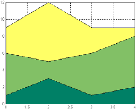
Figure 4-17.
We then create a two-dimensional Comet graph (Figure
4-18
).
>> t = 0:.01:2 * pi;
x = cos(2*t) .* (cos (t) .^ 2);
y = sin(2*t) .* (sin (t) .^ 2);
comet(x,y);
Figure 4-18.
Then is the contour graphic (Figure
4-19
) for the function:
x
xye
1
3
æ
ç
ö
÷
2
,
( )
=-
(
)
2
(
)
-
2
2
2
(
))
-
2
-
x
3
5
- -
x
y
-+
x
1
2
fxy
31
x
e
-+
y
1 0
- -
-
e
y
5
>> f = ['3 *(1-x)^2 * exp (-(x^2)-(y + 1)^2)','-10 *(x/5-x^3-y^5) * exp(-x^2-y^2)',
'-1/3 * exp (-(x + 1)^2 - y^2)'];
>> ezcontour(f,[-3,3],49)