Graphics Reference
In-Depth Information
Figure 3-8.
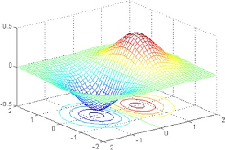
finally, figure
3-9
represent the mesh graphic and curtain option. the syntax is as follows:
>> [X, Y] = meshgrid(-2:.1:2,-2:.1:2);
>>
Z
= X .* exp(-X.^2 -
Y
.^2);
>> meshz(X, Y, Z)
Figure 3-9.
3.7 Contour Graphics
Another option for visualizing a function of two variables is to use level curves calls (a system of dimensional planes.
These curves are characterized as such because they are the points
(x, y)
on which the value of
f(x,y)
is constant.
Thus, for example, in the weather charts, level curves representing the same temperature points are called isotherms,
and contour lines of equal pressure, isobars. Contour lines, representing heights (values of
f(x,y)
that are equivalent,
can describe surfaces in space. Thus, drawing different contours corresponding to constant heights, can be described
as a map of lines on the surface level, MATLAB calls a
contour graph
. The contour plots can be represented in two and
three dimensions.
A map showing the regions of the Earth's surface, whose contour lines represent the height above the sea level,
is called a topographic map. These maps, therefore show the variance of z =
f(x,y)
with respect to
x
and
y
. When the
space between contour lines is large, it means that the variation of the variable
z
is slow, while a small space indicates
a rapid change of
z
.