Graphics Reference
In-Depth Information
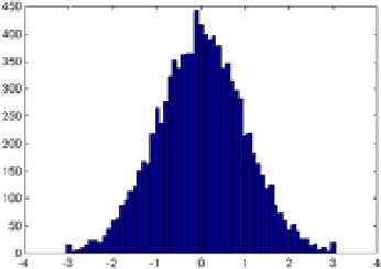
The histogram in Figure
2-21
, corresponds to a vector of 10,000 normal random values in 60 bins between the
values - 3 and 3 in0.1 increments:
>> x = -3:0.1:3;
>> y = randn(10000,1);
>> hist(y,x)
Figure 2-21.
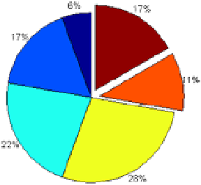
Figure
2-22
is a pie chart with two of its areas displaced, produced by using the syntax:
>> pie([1, 3, 4, 5, 2, 3], [0,0,0,0,1,1])
Figure 2-22.
2.9 Statistical Errors and Arrow Graphics
There are commands in MATLAB which enable charting errors of a function, as well as certain types of arrow graphics
to be discussed now. Some of these commands are described below:
errorbar(x,y,e)
carries out the graph of the vector
x
against the vector
y
with the errors
specified in the vector
e
. Passing through each point
(xi, yi)
draws a vertical line of length
2ei whose center is the point
(xi, yi).
stem(Y)
draws the graph of the vector
Y
cluster. Each point
Y
is attached to the axis
x
by a
vertical line.
stem(X,Y)
draw the graph of the
Y
vector cluster whose elements are given by the vector
X.