Graphics Reference
In-Depth Information
eXerCISe 6-5
Calculate the second degree interpolation polynomial passing through the points (-1,4), (0,2), and (1,6) in the least
squares sense.
>> x=[-1,0,1];y=[4,2,6];p=poly2sym(polyfit(x,y,2))
p =
3 * x ^ 2 + x + 2
eXerCISe 6-6
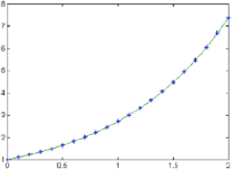
represent 200 points of cubic interpolation between the points (x, y) given by the values that the function takes
exponential e ^ x using 20x values equally spaced between 0 and 2. also represent the difference between the
function e ^ x and its approximation by interpolation. Use cubic interpolation.
First, we define the 20 given points
(x, y)
, equally spaced between 0 and 2:
>> x = 0:0.1:2;
>> y = exp(x);
now we find 200 points
(xi, yi)
for cubic interpolation, equally spaced between 0 and 2, and they are represented
on a graph, together with the 20 points
(x, y)
using asterisks. see Figure
6-1
:
>> xi = 0:0.01:2;
>> yi = interp1(x,y,xi,'cubic');
>> plot(x,y,'*',xi,yi)
Figure 6-1.