Graphics Reference
In-Depth Information
Figure 5-12.
Later is a graphical surface and contour (Figure
5-13
).
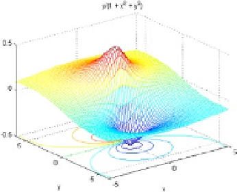
>> ezsurfc('y/(1 + x^2 + y^2)', [- 5, 5, - 2*pi, 2*pi], 35)
Figure 5-13.
Then we graph a curve in parametric space.
>> ezplot3('sin(t)', 'cos(t)',', [0, 6 * pi])
eXerCISe 5-1
represent the following function in the interval [-8.8]
3
x
fx
()=
x
2
-
4
Figure
5-14
represents the function by using the following syntax:
>> ezplot('x^3 / (x^2-4)', [-8, 8])