CONTRIBUTION OF PRESENT RESEARCH TO UNCERTAINTY ASSESSMENT METHODS - Modelling Uncertainty in Flood Forecasting Systems - page 77

where & !=[0,1]. The superscript (*) is used in Equations (4.68) and (4.69) to indicate that
they are modified operations. For the proposed transformation (Equation (4.65)), it is
easy to check that &' =1! & . This makes Equations (4.44) and (4.46) equivalent to
Equations (4.68) and (4.69), respectively for the ! and & related by Equation (4.67).
4.4.4 Application example
In order to illustrate the application of the CDF-MF transformations proposed above, the
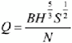
uniform flow formula of the form given by Equation (4.70) is used, i.e.
(4.70)
where Q is the discharge (m 3 /s), B and H are the channel width (m) and water depth (m),
respectively, S is the water surface slope (m/m) and N is the Manning's roughness coefficient
(m !1/3 s). This form of the uniform flow formula assumes a wide rectangular channel with
P = B + 2H & B .
This illustration consists of the following steps:
1. The B, H, S and N are assumed as uncertain input variables, each defined by a bounded
normal PDF. The CDFs of these inputs derived from their PDFs are given in Figure 4.17.
2. The uncertainty in the output Q due to the uncertainty in the inputs is estimated by
applying a modified MC simulation (also referred here as a random simulation).
As required by Equation (4.55) (for multiplication) and Equation (4.69) (for
division), the modified MC simulations are performed in such a way that in each
simulation the same value of a random number (&) is used to sample values of B,
H and S and a random number 1! & is used to sample a value of N . The output
uncertainty in the form of the CDF is shown in Figure 4.18.
3. The CDFs of the inputs are transformed to MFs using the transformation given
by Equation (4.65). The transformed MFs are shown in Figure 4.17.
4. The uncertainty in the output Q is estimated due to the input uncertainty in the
form of MF (transformed from CDF) by applying the fuzzy EP using the ! -cut
method (also referred here as a fuzzy simulation). The output uncertainty in the
form of the MF is shown in Figure 4.19.
5. The output CDF obtained in Step 2 (from random simulation) is transformed to a
MF by applying the transformation defined by Equation (4.65) and compared with
the output MF obtained in Step 4 (from fuzzy simulation) as shown in Figure 4.18.
6. Similarly, the output MF obtained in Step 4 is transformed to a CDF by applying
the transformation defined by Equation (4.66) and compared with the
output CDF obtained in Step 2 as shown in Figure 4.19.
The comparisons show that the results are in perfect agreement. An implication of this
result is that it provides an alternative method for the evaluation of the Extension
Principle for a monotonic function without using the ! -cut method.