Image Processing Reference
In-Depth Information
A fast version of the DCT is available, like the FFT, and calculation can be based on the
FFT. Both implementations offer about the same speed. The Fourier transform is not
actually optimal for
image coding
since the Discrete Cosine transform can give a higher
compression rate, for the same image quality. This is because the cosine basis functions
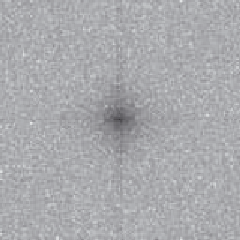
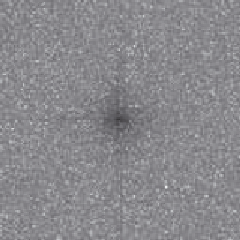
can afford for high energy compaction. This can be seen by comparison of Figure
2.21
(b)
with Figure
2.21
(a), which reveals that the DCT components are much more concentrated
around the origin, than those for the Fourier transform. This is the compaction property
associated with the DCT. The DCT has actually been considered as optimal for image
coding, and this is why it is found in the JPEG and MPEG standards for coded image
transmission.
(a) Fourier transform
(b) Discrete cosine transform
(c) Hartley transform
Figure 2.21
Comparing transforms of lena
The DCT is actually shift variant, due to its cosine basis functions. In other respects, its
properties are very similar to the DFT, with one important exception: it has not yet proved
possible to implement convolution with the DCT. It is actually possible to calculate the
DCT via the FFT. This has been performed in Figure
2.21
(b) since there is no fast DCT
algorithm in Mathcad and, as shown earlier, fast implementations of transform calculation
can take a fraction of the time of the conventional counterpart.
The Fourier transform essentially decomposes, or
decimates
, a signal into sine and
cosine components, so the natural partner to the DCT is the Discrete Sine Transform
(DST). However, the DST transform has odd basis functions (sine) rather than the even
ones in the DCT. This lends the DST transform some less desirable properties, and it finds
much less application than the DCT.
2.7.2
Discrete Hartley transform
The Hartley transform (Hartley, 1942) is a form of the Fourier transform, but without
complex arithmetic, with result for the face image shown in Figure
2.21
(c). Oddly, though
it sounds like a very rational development, the Hartley transform was first invented in
1942, but not rediscovered and then formulated in discrete form until 1983 (Bracewell,
1983). One advantage of the Hartley transform is that the forward and inverse transform