Images, sampling and frequency domain processing - Feature Extraction and Image Processing - page 52

implies that the centre of a transform image will now be the d.c. component. (Another way
of interpreting this is rather than look at the frequencies centred on where the image is, our
viewpoint has been shifted so as to be centred on one of its corners - thus invoking the
replication property.) The operator rearrange , in Code 2.2 , is used prior to transform
calculation and results in the image of Figure 2.15 (c), and all later transform images.

for y ∈ 0..rows(picture)-1
for x ∈ 0..cols(picture)-1
rearranged_pic y,x ← picture y,x ·(-1) (y+x)
rearranged_pic

rearrange(picture):=

Code 2.2 Reordering for transform calculation

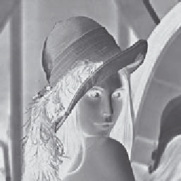
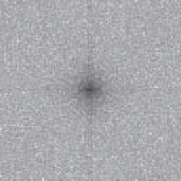
The full effect of the Fourier transform is shown by application to an image of much
higher resolution. Figure 2.16 (a) shows the image of a face and Figure 2.16 (b) shows its
transform. The transform reveals that much of the information is carried in the lower
frequencies since this is where most of the spectral components concentrate. This is because
the face image has many regions where the brightness does not change a lot, such as the
cheeks and forehead. The high frequency components reflect change in intensity. Accordingly,
the higher frequency components arise from the hair (and that feather!) and from the
borders of features of the human face, such as the nose and eyes.

(a) Image of face (b) Transform of face image

Figure 2.16 Applying the Fourier transform to the image of a face

As with the 1D Fourier transform, there are 2D Fourier transform pairs, illustrated in
Figure 2.17 . The 2D Fourier transform of a two-dimensional pulse, Figure 2.17 (a), is a
two-dimensional sinc function, in Figure 2.17 (b). The 2D Fourier transform of a Gaussian
function, in Figure 2.17 (c), is again a two-dimensional Gaussian function in the frequency
domain, in Figure 2.17 (d).