Image Processing Reference
In-Depth Information
which, at first, is difficult to interpret. The Fourier transform of an image gives the frequency
components. The position of each component reflects its frequency:
low
frequency components
are
near
the origin and
high
frequency components are further
away
. As before, the lowest
frequency component - for zero frequency - the d.c. component represents the
average
value of the samples. Unfortunately, the arrangement of the 2D Fourier transform places
the low frequency components at the
corners
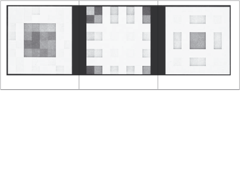
of the transform. The image of the square in
Figure
2.15
(a) shows this in its transform, Figure
2.15
(b). A spatial transform is easier to
visualise if the d.c. (zero frequency) component is in the
centre
, with frequency increasing
towards the edge of the image. This can be arranged either by rotating each of the four
quadrants in the Fourier transform by 180° . An alternative is to
reorder
the original image
to give a transform which shifts the transform to the centre. Both operations result in the
image in Figure
2.15
(c) wherein the transform is much more easily seen. Note that this is
aimed to improve visualisation and does not change any of the frequency domain information,
only the way it is displayed.
(a) Image of square
(b) Original DFT
(c) Rearranged DFT
Figure 2.15
Rearranging the 2D DFT for display purposes
To rearrange the image so that the d.c. component is in the centre, the frequency
components need to be reordered. This can be achieved simply by multiplying each image
point
P
x
,
y
by -1
(
x
+
y
)
. Since cos(-π ) = -1, then -1 =
e
-
j
π
(the minus sign in the exponent
keeps the analysis neat) so we obtain the transform of the multiplied image as:
2
2
N
-1
N
-1
N
-1
N
-1
v
v
-
j
(+)
ux
y
-
j
(+)
-(+)
ux
y
1
=
1
N
N
P
e
- 1
(+)
xy
P
e
e
j
xy
N
x,y
N
x,y
x
=0
y
=0
x
=0
y
=0
2
N
N
N
-1
N
-1
-
j
u
+
2
x
++
2
v
y
=
1
N
P
e
(2.28)
N
x,y
x
=0
y
=0
=
FP
u
N
+
N
v
+
2
,
2
According to Equation 2.28, when pixel values are multiplied by -1
(
x
+
y
)
, the Fourier
transform becomes shifted along each axis by half the number of samples. According to the
replication theorem, Equation 2.26, the transform replicates along the frequency axes. This