Image Processing Reference
In-Depth Information
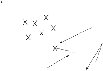
two-dimensional feature space produced by the two measures made on each sample, measure
1 and measure 2. Each sample gives different values for these measures but the samples of
different classes give rise to clusters in the feature space where each cluster is associated
with a single class. In Figure
8.5
we have seven samples of two known textures: Class A
and Class B depicted by
and
, respectively. We want to classify a test sample, depicted
by
+
, as belonging either to Class A or to Class B (i.e. we assume that the training data
contains representatives of all possible classes). Its nearest neighbour, the sample with
least distance, is one of the samples of Class A so we could then say that our test appears
to be another sample of Class A (i.e. the class label associated with it is Class A). Clearly,
the clusters will be far apart for measures that have good discriminatory ability whereas the
clusters will overlap for measures that have poor discriminatory ability. That is how we can
choose measures for particular tasks. Before that, let us look at how best to associate a
class label with our test sample.
Measure 2
7 samples (X)
of class A
Nearest neighbour
3-nearest neighbours
7 samples (O)
of class B
Test sample
Measure 1
Figure 8.5
Feature space and classification
Classifying a test sample as the training sample it is closest to in feature space is
actually a specific case of a general classification rule known as the
k-nearest neighbour
rule
. In this rule, the class selected is the
mode
of the sample's nearest
k
neighbours. By the
k
-nearest neighbour rule, for
k
= 3, we select the nearest three neighbours (those three with