Image Processing Reference
In-Depth Information
250
200
6
150
4
100
2
50
0
0
50
100
150
200
250
300
0
0
50
100
150
200
250
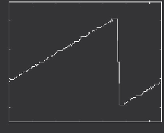
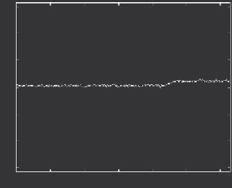
(a) Curve
(b) Angular function
1
0
6
4
-1
2
-2
-3
0
-4
-2
-5
-4
-6
-7
-6
0
50
100
150
200
250
300
0
1
2
3
4
5
6
(c) Cumulative
(d) Normalised
Figure 7.12
Discrete computation of the angular functions
=
2
π
dt
ds
(7.33)
L
Accordingly, the coefficients in Equation 7.32 can be rewritten as,
L
= 2 +
2
*
a
()
sds
L
0
L
2
k
=
2
a
*
( ) cos
s
sds
(7.34)
k
L
L
0
L
2
k
= -
2
+
2
*
b
( ) sin
s
sds
k
k
L
L
0
In a similar way to Equation 7.26, the Fourier descriptors can be computed by approximating
the integral as a summation of rectangular areas. This is illustrated in Figure
7.13
. Here, the
discrete approximation is formed by rectangles of length τ
i
and height γ
i
. Thus,