Image Processing Reference
In-Depth Information
Thus, if we have
m
sampling points, then the sampling period is equal to τ
=
T
/
m
. Accordingly,
the maximum frequency in the approximation is given by
m
T
f
c
=
2
(7.22)
Each term in Equation 7.11 defines a trigonometric function at frequency
f
k
=
k
/
T
. By
comparing this frequency with the relationship in Equation 7.15, we have that the maximum
frequency is obtained when
m
k
=
2
(7.23)
Thus, in order to define a smooth curve that passes through the
m
regularly-sampled points,
we need to consider only
m
/2 coefficients. The other coefficients define frequencies higher
than the maximum frequency. Accordingly, the Fourier expansion can be redefined as
m
/2
a
0
(7.24)
ct
() =
+
(
a
cos(
k
t
) +
b
sin(
k
t
))
k
k
2
k
=1
In practice, Fourier descriptors are computed for fewer coefficients than the limit of
m
/2.
This is because the low frequency components provide most of the features of a shape.
High frequencies are easily affected by noise and only represent detail that is of little value
to recognition. We can interpret Equation 7.22 the other way around: if we know the
maximum frequency in the curve, then we can determine the appropriate number of samples.
However, the fact that we consider
c
(
t
) to define a continuous curve implies that in order
to obtain the coefficients in Equation 7.13, we need to evaluate an integral of a continuous
curve. The approximation of the integral is improved by increasing the sampling points.
Thus, as a practical rule, in order to improve accuracy, we must try to have a large number
of samples even if it is theoretically limited by the Nyquist theorem.
Our curve is only a set of discrete points. We want to maintain a continuous curve
analysis in order to obtain a set of discrete coefficients. Thus, the only alternative is to
approximate the coefficients by approximating the value of the integrals in Equation 7.13.
We can approximate the value of the integral in several ways. The most straightforward
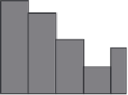
approach is to use a Riemann sum. Figure
7.9
illustrates this approach. In Figure
7.9
(b), the
integral is approximated as the summation of the rectangular areas. The middle point of
each rectangle corresponds to each sampling point. Sampling points are defined at the
points whose parameter is
t
=
i
τ where
i
is an integer between 1 and
m
. We consider that
c
i
defines the value of the function at the sampling point
i
. That is,
c(t) cos(k
t)
(T/m)c
i
cos(k
ω
)
(T/m)c
i
cos(k
ω
)
i
i
0
T
0
T
0
T
(a) Continuous curve
(b) Rieman sum
(c) Linear interpolation
Figure 7.9
Integral approximation