Image Processing Reference
In-Depth Information
ω
T
. In general, we can define the points [ω
j
, ω
T
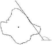
] in different ways. An alternative geometric
arrangement is shown in Figure
5.23
(a). Given the points ω
i
and a fixed angle
, then we
determine the point ω
j
such that the angle between the tangent line at ω
j
and the line that
joins the points is
. The third point is defined by the intersection of the tangent lines at
ω
i
and ω
j
. The tangent of the angle β is defined by Equation 5.88. This can be expressed
in terms of the points and its gradient directions as
-
1 +
φ
φ φ
i
j
Q
() =
(5.89)
i
i
j
We can replace the gradient angle in the R-table by the angle
. The form of the new
invariant table is shown in Figure
5.23
(c). Since the angle
does not change with rotation
or change of scale, then we do not need to change the index for each potential rotation and
scale. However, the displacement vector changes according to rotation and scale (i.e.
Equation 5.85). Thus, if we want an invariant formulation, then we must also change the
definition of the position vector.
T
ω
j
k
ω
i
0
k
0
, k
1
, k
2
, ...
ˆ
θ
()
j
(x
0
,y
0
)
i
M
k
2
∆φ
M
ˆ
θ
()
…
…
ˆ
θ
()
i
ˆ
θ
()
(a) Displacement vector
(b) Angle definition
(c) Invariant R-table
Figure 5.23
Geometry of the invariant GHT
In order to locate the point
b
we can generalise the ideas presented in Figure
5.17
(a) and
Figure
5.19
(a). Figure
5.23
(b) shows this generalisation. As in the case of the circle and
ellipse, we can locate the shape by considering a line of votes that passes through the point
b
. This line is determined by the value of
φ
i
. We will do two things. First, we will find an
invariant definition of this value. Second, we will include it on the GHT table.
We can develop Equation 5.73 as
x
y
cos (
)
sin(
)
x
y
(
()
)
xi
0
(5.90)
=
+
- sin (
)
cos (
)
yi
0
Thus, Equation 5.60 generalises to
-
-
y
x
=
[- sin
(
) cos(
)]
y
x
(
)
yi
xi
0
0
=
(5.91)
i
[cos(
) sin (
)]
(
)
By some algebraic manipulation, we have that
(5.92)
i
= tan( - )