what-when-how
In Depth Tutorials and Information
1
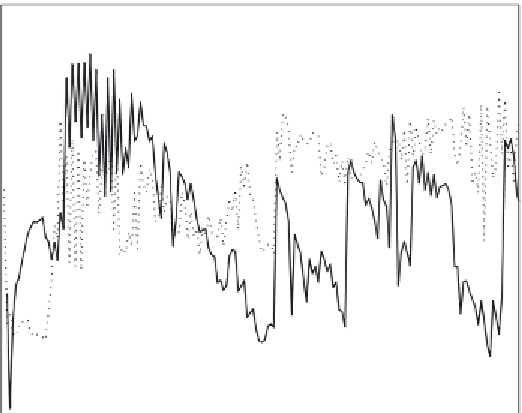
Connection
Interest
Unchoked
Download
0.9
0.8
0.7
0.6
0.5
0.4
0.3
0.2
0.1
0
5
10
15
20
25
30
35
40
45
Time (hours)
Figure 6.12
The goodness of it (
R
2
) parameter measured during the
experiments.
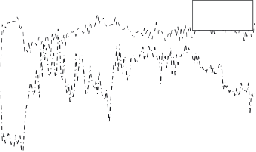
to vary quite a lot during the initial stage. However, once all the peers have joined
the system the power law exponent quickly reaches its final value, and remains very
steady at just over 2 through most of the transient stage and all of the steady stage.
6.3.3 Small-World Networks: Negative Results
he concept of a small-world phenomenon was first introduced by Milgram [25] to
refer to the principle that people are linked to all others by short chains of acquain-
tances (popularly known as
sixdegreesofseparation
). his formulation was used by
Watts and Strogatz to describe networks that are neither completely random, nor
completely regular, but possess characteristics of both [31,30]. hey introduce a
measure of one of these characteristics, the cliquishness of a typical neighborhood,
as the
clusteringcoeicient
of the graph. hey deine a small-world graph as one in
which the clustering coefficient is still large, as in regular graphs, but the measure
of the average distance between nodes, the
characteristicpathlength
, is small as in
random graphs.
Given a graph
G
= (
V
,
E
), the clustering coefficient
Ci
of a node
i
Î
V
is the
proportion of all the possible edges between neighbors of the node that actually
exist in the graph. A sample graph showing a single node's neighbors and its clus-
tering coefficient is shown in Figure 6.14. For a node
i
of degree
k
i
, the maximum