Image Processing Reference
In-Depth Information
Table 4.1
A small histogram and its cumulative histogram.
i
is the bin number,
H
[
i
]
the height of bin
i
,and
C
[
i
]
is the height of the
i
thbininthecumulative
histogram
i
0
1
2
3
H
[
i
]
1
5
0
7
C
[
i
]
1
6
6
13
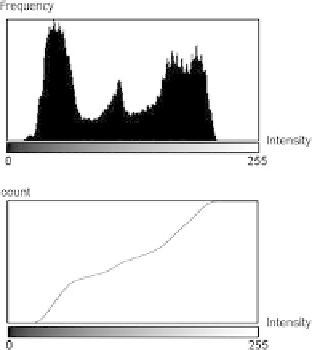
Fig. 4.14
An example of a
cumulative histogram. Notice
how the tall bins in the
ordinary histogram translate
into steep slopes in the
cumulative histogram
Imagine we have a histogram
H
[
i
]
where
i
is a bin number (between 0 and 255)
and
H
[
i
]
is the height of bin
i
. The cumulative histogram is then defined as
j
C
[
j
]=
H
[
i
]
(4.12)
i
=
0
In Table
4.1
a small example is provided.
In Fig.
4.14
a histogram is shown together with its cumulative histogram. Where
the histogram has high bins, the cumulative histogram has a steep slope and where
the histogram has low bins, the cumulative histogram has a small slope. The idea is
now to use the cumulative histogram as a gray-level mapping. So the pixel values
located in areas of the histogram where the bins are high and dense will be mapping
to a wider interval in the output since the slope is above 1. On the other hand, the
regions in the histogram where the bins are small and far apart will be mapped to a
smaller interval since the slope of the gray-level mapping is below 1.
For this to work in practice we need to ensure that the y-axis of the cumulative
histogram is in the range
. This is simply done by first dividing each value on
the y-axis with
count
, i.e., the total number of pixels in the image, and then multiply
with 255. In Fig.
4.15
the effect of histogram equalization is illustrated.
[
0
,
255
]