Image Processing Reference
In-Depth Information
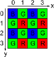
Fig. 3.5
The Bayer pattern
used for capturing a color
image on a single image
sensor. R
=
red, G
=
green,
and B
=
blue
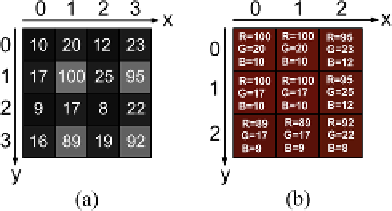
Fig. 3.6
(
a
) Numbers
measured by the sensor.
(
b
) Estimated RGB image
using Eq.
3.2
the result. How to balance these two issues is up to the camera manufactures, and
in general, the higher the quality of the camera, the higher the cost. Even very ad-
vanced algorithms are not as good as a three sensor color camera and note that when
using, for example, a cheap web-camera, the quality of the colors might not be too
good and care should be taken before using the colors for any processing. Regard-
less of the choice of demosaicing algorithm, the output is the same as when using
three sensors, namely Eq.
3.1
. That is, even though only one color is measured per
pixel, the output for each pixel will (after demosaicing) consist of three values: R,
G, and B.
An example of a simple demosaicing algorithm is to infer the missing colors
from the nearest pixels, for example using the following set of equations:
⎧
⎨
[
R,G,B
]
B
=[
f(x
+
1
,y
+
1
), f (x
+
1
,y),f(x,y)
]
[
R,G,B
]
GB
=[
f(x,y
+
1
),f(x,y),f (x
−
1
,y)
]
g(x,y)
(3.2)
⎩
[
R,G,B
]
GR
=[
f(x
+
1
,y),f(x,y),f(x,y
−
1
)
]
[
R,G,B
]
R
=[
f(x,y),f (x
−
1
,y),f(x
−
1
,y
−
1
)
]
where
f(x,y)
is the input image (Bayer pattern) and
g(x,y)
is the output RGB
image. The RGB values in the output image are found differently depending on
which color a particular pixel is sensitive to:
[
R,G,B
]
B
should be used for the
pixels sensitive to blue,
[
R,G,B
]
R
should be used for the pixels sensitive to red,
and
]
GR
should be used for the pixels sensitive to green
followed by a blue or red pixel, respectively.
In Fig.
3.6
a concrete example of this algorithm is illustrated. In the left figure
the values sampled from the sensor are shown. In the right figure the resulting RGB
output image is shown using Eq.
3.2
.
[
R,G,B
]
GB
and
[
R,G,B