Image Processing Reference
In-Depth Information
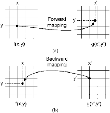
Fig. 10.2
(
a
)Forward
mapping. (
b
) Backward
mapping
10.2 Making It Work in Practice
In terms of programming, the affine transformation consists of two steps. First the
coefficients of the affine transformation matrix are defined. Second we go though all
pixels in the image
f(x,y)
one at a time (using two for-loops as seen in Sect. 4.7)
and for each pixel we find its new position in
g(x
,y
)
using Eq.
10.9
. This process
is known as
forward mapping
, i.e., mapping each pixel from
f(x,y)
to
g(x
,y
)
,
see Fig.
10.2
(a).
At first glance this simple process seems to be fine, but unfortunately it is not
!Let
us have a closer look at the scaling transformation in order to understand the nature
of the problem. Say we have an image of size 300
×
200 and want to scale this to
510
×
200. From above we can calculate the scaling factors as
S
x
=
510
/
300
=
1
.
7
and
S
y
=
1. Using Eq.
10.4
the pixel positions in a row of
f(x,y)
are
mapped in the following manner:
200
/
200
=
x
0
1
2
3
4
5
6
7
8
···
300
x
0
1.7
3.4
5.1
6.8
8.5
10
.
2
11
.
9
13
.
6
···
510
We can observe that “holes” are present in
g(x
,y
)
. If for example 10.2 is
rounded off to 10 and 11.9 to 12, then
x
=
11 will have no value, hence a hole
in the image output. In Fig.
10.3
we have used forward mapping to scale image
10.1
(a). The holes can be seen as the black pattern.
If the scaling factor is smaller than 1 then a related problem would occur, namely
that multiple pixels from
f(x,y)
are mapped to the same pixel in
g(x
,y
)
.Thisis
not critical in terms of how the output would look like, but mapping multiple pixels
to the same pixel in
g(x
,y
)
is computationally inefficient. Both these issues are
present in all geometric transformations.