Image Processing Reference
In-Depth Information
Table 9.1
The position of an object over time
i
e
1
2
3
4
5
6
7
8
9
10
11
12
13
···
X
1
2
4
5
4
6
8
9
9
7
3
2
2
···
Y
10
8
8
7
6
4
4
3
2
2
2
2
4
···
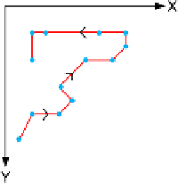
Fig. 9.1
The trajectory of an
object over time
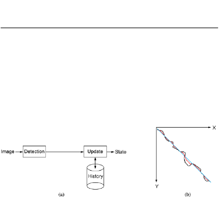
Fig. 9.2
(
a
) Framework for updating the state. (
b
) The effect of updating the states. The
blue curve
is the true trajectory of the object. The
black curve
is the detected trajectory and the
red curve
is
the smoothed trajectory
Smoothing can be implemented by calculating the average of the last
N
states.
The larger
N
is, the more smooth the trajectory will be. As
N
increases so does
the latency in the system, meaning that the updated state will react slow to rapid
position changes. For example if you are tracking a car that is accelerating hard or is
doing an emergency break. This slow reaction can be counteracted by also including
future states in the update of the current state, but such an approach will delay the
output from the system. Whether this is acceptable or not depends on the applica-
tion. Another way of counteracting the latency is to use a weighted smoothing filter.
Instead of adding
N
positions together and dividing by
N
, we weight each position
according to its age. So the current state has the highest weight, the second newest
state has the second highest weight etc. No matter which smoothing method is used
to update the state, it is a compromise between smoothness and latency. In Fig.
9.2
the updating of the state is illustrated. The history-block contains previous states.