Geoscience Reference
In-Depth Information
2
P
1
3
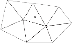
Fig. 9.3. Geometric interpolation
we assign its value ∆
g
as its
z
-coordinate, so that the points 1, 2, and 3
have “spatial” coordinates (
x
1
,y
1
,z
1
), (
x
2
,y
2
,z
2
), and (
x
3
,y
3
,z
3
);
x
and
y
are ordinary plane coordinates. The plane through 1, 2, 3 has the equation
(
x
2
−
x
)(
y
3
−
y
2
)
−
(
y
2
−
y
)(
x
3
−
x
2
)
z
=
x
2
)
z
1
(
x
2
−
x
1
)(
y
3
−
y
2
)
−
(
y
2
−
y
1
)(
x
3
−
(
x
3
−
x
)(
y
1
−
y
3
)
−
(
y
3
−
y
)(
x
1
−
x
3
)
+
x
3
)
z
2
(9-42)
(
x
3
−
x
2
)(
y
1
−
y
3
)
−
(
y
3
−
y
2
)(
x
1
−
(
x
1
−
x
)(
y
2
−
y
1
)
−
(
y
1
−
y
)(
x
2
−
x
1
)
+
x
1
)
z
3
.
(
x
1
−
x
3
)(
y
2
−
y
1
)
−
(
y
1
−
y
3
)(
x
2
−
If we replace
z
1
,z
2
,z
3
by ∆
g
1
,
∆
g
2
,
∆
g
3
,then
z
is the interpolated value
∆
g
P
at point
P
, which has the plane coordinates
x, y
.Thus,
∆
g
P
=
α
P
1
∆
g
1
+
α
P
2
∆
g
2
+
α
P
3
∆
g
3
,
(9-43)
where the
α
Pi
are the coecients of
z
i
in the preceding equation.
Representation
Often the measured anomaly of a gravity station 1 is made to represent the
whole neighborhood so that
∆
g
P
≡
∆
g
1
(9-44)
as long as P lies within a certain neighborhood of point 1. Then
α
P
1
=1
,
P
2
=
α
P
3
=
...
=
α
Pn
=0
.
(9-45)
This method is rather crude but simple and accurate enough for many pur-
poses.