Information Technology Reference
In-Depth Information
2
is the Laplacian, and
D
V
is the
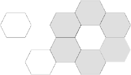
diffusion coecient. The simulation is run on a hexagonal grid. The geometry
of the grid and the base vectors we chose are illustrated in Fig. 2.
where
V
is the concentration of virions,
∇
3
4
Δ
x
(
m, n −
1)
m
1
2
Δ
x
n
Δ
x
(
m −
1
,n
)
(
m
+1
,n−
1)
(
m, n
)
(
m −
1
,n
+1)
(
m
+1
,n
)
(
m, n
+1)
Fig. 2.
Geometry of agent-based model's hexagonal grid. The honeycomb neighborhood
is identified in gray, and the base vectors
m
and
n
are shown and expressed as a function
of
Δx
, the grid spacing which is the mean diameter of an epithelial cell.
We can express (1) as a difference equation in the hexagonal coordinates
(
m, n
) as a function of the 6 honeycomb neighbors as
6
nei
V
t
+1
m,n
V
m,n
−
4
D
V
(
Δx
)
2
V
m,n
+
1
V
nei
=
−
,
(2)
Δt
such that
V
t
+1
m,n
at time
t
+1 as a function of
V
m,n
and its 6 honeycomb neighbors
V
nei
at time
t
is given by
m,n
=
1
(
Δx
)
2
V
m,n
+
2
D
V
Δt
3(
Δx
)
2
nei
4
D
V
Δt
V
t
+1
V
nei
,
−
(3)
where
nei
V
nei
is the sum of the virion concentration at all 6 honeycomb neigh-
bors at time
t
.
Because we want to simulate the infection dynamics in an experimental well,
we want the diffusion to obey reflective boundary conditions along the edge
of the well. Namely, we want
∂V
∂j
= 0 at a boundary where
j
is the direction
perpendicular to the boundary. It can be shown that for such a case, (3) becomes
m,n
=
1
V
m,n
+
2
D
V
Δt
3(
Δx
)
2
N
nei
N
nei
2
D
V
Δt
3(
Δx
)
2
V
t
+1
V
N
nei
−
,
(4)