Information Technology Reference
In-Depth Information
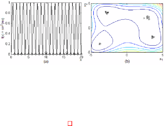
Fig. 3.
The final
-nondominated solutions for (a)
f
(
x
)=sin
2
(
πx
)and(b)Himmel-
blau's function
The second problem is known as Himmelblau's function and is given by:
Minimize
f
(
x
1
,x
2
)=(
x
1
+
x
2
−
11)
2
+(
x
1
+
x
2
−
7)
2
,
−
5
≤
x
1
,x
2
≤
5
.
(5)
For this problem, there are four minima, each having a functional value equal
to zero. As can be seen in Figure 3-b, the regions of these minima concentrated
the final solutions found by the algorithm (31 solutions). The parameters used
were 60 generations, 50 individuals in the initial population, 20 individuals in
Random Insertion, a suppression threshold of 0
.
005, 5 clones per individual and
δ
=0
.
05. During the execution of omni-aiNet, the population size decreased
with the convergence of the algorithm, finishing with 31 individuals (including
the four solutions) whose distance among each other is within the predefined
suppression threshold.
Again, the results presented in Figure 3 seems very promising, once for both
problems the algorithm was capable of identifying the global solutions with a
fine tuning of the population size according to the demand.
6.3
Multi-objective Uni-global Problems
Two problems were selected as test functions for the multi-objective uni-global
problem category: the 30-variable ZDT1 test function, that has a convex Pareto
Front and the 30-variable ZDT2 test function, that is the nonconvex counterpart
to ZDT1. The details of each problem can be found in [13]. Figures 4 and 5
present the true Pareto front (solid lines) and the Pareto front found by (a)
the omni-aiNet; and (b) DT omni-optimizer algorithm for problems ZDT1 and
ZDT2, respectively. The parameters used for omni-aiNet were 50 generations,
100 individuals in the initial population, 10 generations between suppressions, 5
individuals in Random Insertion, a suppression threshold of 0
.
001, 3 clones per
individual and
δ
=0
.
01. For the DT omni-optimizer, it was used
δ
=0
.
01, 100
generations and a population of 100 individuals.
As can be seen in Figures 4 and 5, for both problems the omni-aiNet produced
a final population of solutions much closer to the real Pareto front and with a
better coverage of this front than the DT omni-optimizer.