Graphics Reference
In-Depth Information
Original image
x
coordinate
Minimum image
I
min
x
coordinate
Maximum image
I
max
x
coordinate
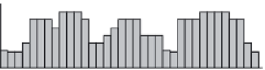
Figure 5.7
Pixel-matching probability is accelerated by precomputing the maximum and minimum
pixel values in the neighborhood at each pixel. These plots show pixel values of the original
images and the computed maximum and minimum images along a horizontal line of pixels.
(From [Sand and Teller 04]
c
2004 ACM, Inc. Included here by permission.)
dence method described above, except that instead of comparing corresponding
pixels in the neighborhood, a pixel in the primary image is compared to a 3
3
neighborhood of pixels at a candidate location in the secondary image. The au-
thors employ a trick to do this efficiently. The minimum and maximum pixel
values in the 3
×
3 neighborhood are precomputed as a kind of filter on the sec-
ondary image; the results are “maximum” and “minimum” images that contain
the precomputed local maxima and minima. Figure 5.7 illustrates these over a
representative slice of an image. From these images, the value of
×
∑
(
,
(
,
)
−
(
+
,
+
)
,
(
+
,
+
)
−
(
,
))
max
0
I
x
y
I
max
x
u
y
v
I
min
x
u
y
v
I
x
y
(
x
,
y
)
∈
R
instead of the square of the pixel differences is minimized over all
.The
computation is repeated for each color channel independently. From this a pixel-
matching probability is computed, and the pixel is omitted from the correspon-
dence if it is deemed unlikely to match any pixel in the secondary image. Doing
this makes the algorithm more robust, as small mismatches have limited effect on
the final matching. If the match is considered likely, the offset vector
(
u
,
v
)
(
u
,
v
)
of the
pixel is recorded along with the matching probability.
One problem with any pixel-matching approach arises in regions of the im-
age where there is little variation between pixel values, i.e., in areas of uniform
color. The file folder on the right in the images of Figure 5.6 is a good example;