Graphics Reference
In-Depth Information
2
x
2
x
I
1
I
0
→
d
(
dx
,
dy
)
q(
x
+
dx
,
y
+
dy
)
2
y
(
x
,
y
)
2
y
(a)
(b)
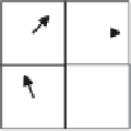
Figure 5.4
Corresponding neighborhoods in (a) the primary image and (b) the secondary image.
The correction vector computation thus reduces to a least squares problem that
can be solved by standard methods. Other approaches use image gradients or
higher-order approximations to how the pixels actually change.
An
image pyramid
method can be employed to improve optical flow compu-
tation. The original images are repeatedly downsampled to create a sequence of
images of decreasing size that can be thought of as a kind of pyramid (
Figure 5.5
)
.
Much like the construction of a mip map (Chapter 3), each pixel is the average of
a block of four pixels at the previous level. Each image in the sequence therefore
has half the resolution of the previous image. A pyramid is constructed for both
images
I
0
and
I
1
. The offset vector field computation is applied at each level of the
pyramid starting at the top. At the top level, where the image has been reduced to
Optical flow
computed at Level 3
Level 3
Level 2
Level 0
(original image)
Level 1
Level 0
Level 1
Double the resolution
Optical flow
computed at Level 2
Recompute
optical flow
(update)
Level 2
Level 3
Halve the resolution
at each level
Figure 5.5
Optical flow can be made more efficient and stable with an image pyramid constructed
by repeatedly downsampling the image by a factor of two (right). The optical flow is
determined first at the top level, and the result is replicated on the pixels in the next level
(left) which are then recomputed or refined.