Simulation of flow and sediment transport in vegetated channels - Computational River Dynamics - page 395

Figure 10.10 (a) Mean velocities, (b) Reynolds shear stresses, and (c) streamwise turbulence
intensities of flow over submerged vegetation (Shimizu and Tsujimoto, 1994).

However, because the k - turbulence models usually may not compute the

streamwise turbulence intensity or normal stress accurately, it is necessary to cali-
brate the two coefficients using the measurement data of other quantities, such as
the turbulent energy k , that these turbulence models can handle well. Before this is
done, it is the modeler's preference to use which set of c fk and c f ε values. To this
author, it is more comfortable to use c fk =

ε and k - ω

1.0 and c f ε = 1.33 since they are derived

theoretically.
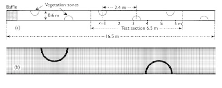
The second example cited here is the simulation of flow around alternate vegetation
zones done by Wu and Wang (2004b) using the depth-averaged 2-D model described
above. The experiments were conducted by Bennett et al . (2002) in a 16.5m long tilting
recirculating flume. Six semi-circular vegetation zones with an equal spacing of 2.4 m
were distributed alternately to achieve a meandering pattern, as shown in Fig. 10.11(a).
The diameter of the vegetation zones was 0.6 m. The model vegetation was emergent
wooden dowel with a diameter of 3.2 mm, laid out in a staggered pattern in each
vegetation zone. Five vegetation concentrations of 0.04%, 0.2%, 0.6%, 2.5%, and
10% were used. The flow discharge was 0.0043 m 3 s − 1 , and the pre-vegetation flow
depth was 0.027 m. The slope of the flume was 0.0004. The surface flow velocity was
measured using the Particle Image Velocimetry (PIV) technique. The computational

Figure 10.11 (a) Plan view and (b) mesh for experiments of Bennett et al . (2002).