Geoscience Reference
In-Depth Information
For a wave structure like Fig. 9.3 or 9.4, the basic WAF method gives the intercell
flux as
N
+
1
w
k
F
(
k
)
F
i
+
1
/
2
=
(9.44)
i
+
1
/
2
k
=
1
where
w
k
is the weight given by
1
2
(
w
k
=
c
k
−
c
k
−
1
)
(9.45)
with
c
k
as the Courant number for wave
k
,
c
k
=
S
k
/
x
,
c
0
=−
1, and
c
N
+
1
=
1.
Here,
S
k
is the speed of wave
k
, and
N
is the number of conservation laws or the
number of waves in the solution of the Riemann problem.
F
(
k
)
i
t
2
is the value of the
+
1
/
(
(
k
)
i
flux vector
F
in the interval
k
of length
w
k
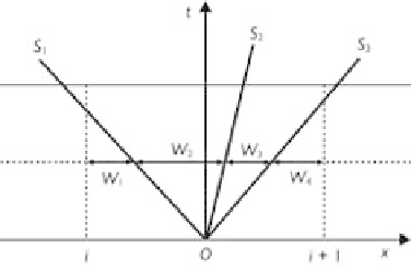
shown in Fig. 9.5, and can be
determined using Eq. (9.18) or (9.22). Inserting Eq. (9.45) into Eq. (9.44) yields an
alternative expression:
)
+
1
/
2
N
1
2
(
1
2
F
(
k
)
i
F
i
+
1
/
2
=
F
i
+
F
i
+
1
)
−
c
k
(9.46)
+
1
/
2
k
=
1
F
(
k
)
i
F
(
k
+
1
)
i
F
(
k
)
i
where
2
is the flux jump across wave
k
.
For a linear convection equation, the WAF scheme (9.46) reproduces identically the
Lax-Wendroff method, which is second-order accurate in space and time. Spurious
oscillations in the vicinity of high gradients are expected. Such non-physical oscillations
can be avoided by enforcing the TVD constraint on the scheme. The TVD version of
the WAF scheme is
=
−
+
1
/
2
+
1
/
2
+
1
/
N
1
2
(
1
2
F
(
k
)
i
F
i
+
1
/
2
=
F
i
+
F
i
+
1
)
−
sign
(
c
k
)
A
k
(9.47)
+
1
/
2
k
=
1
Figure 9.5
Weights in the WAF scheme.