Geoscience Reference
In-Depth Information
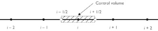
Figure 9.1
1-D finite volume mesh.
Applying the Green theorem to Eq. (9.9) and using the Euler scheme for the time
derivative results in the following discretized equation:
−
t
n
+
1
n
i
F
i
+
1
/
2
−
F
i
−
1
/
2
)
+
t
S
i
=
x
i
(
(9.10)
i
where
F
i
+
1
/
2
is the intercell flux at face
i
+
1
/
2,
x
i
is the length of the
i
th control
volume,
t
is the time step, and the superscript
n
is the time step index.
A rectangular (quadrilateral) or triangular mesh may be used in the numerical
solution of the 2-D shallow water equations. For simplicity, the rectangular mesh
shown in Fig. 9.2 is used here. Integrating Eq. (9.5) over the 2-D control volume
numbered as (
i
,
j
) and using the Euler scheme for the time derivative yields the following
discretized equation:
−
t
F
i
−
1
/
2,
j
)
−
t
n
+
1
n
i
,
j
F
i
+
1
/
2,
j
−
G
i
,
j
+
1
/
2
−
G
i
,
j
−
1
/
2
)
+
t
S
i
,
j
=
x
i
,
j
(
y
i
,
j
(
(9.11)
i
,
j
where
x
i
,
j
and
y
i
,
j
are the lengths of the control volume in the
x
- and
y
-directions,
respectively.
Figure 9.2
2-D finite volume mesh.