Geoscience Reference
In-Depth Information
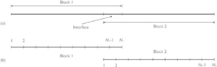
Figure 8.3
(a) Domain decomposition and (b) grid arrangement in a 1-D model.
of block 1, the boundary value of
φ
1,
N
1
is unknown, and in the solution of block 2,
the boundary value of
φ
2,1
is unknown. They can be interpolated using the values of
φ
on the other block by the following interpolation schemes:
L
2
φ
=
L
1
γ
φ
2,
j
, 1
≤
L
1
≤
L
2
≤
N
2
(8.2a)
1,
N
1
j
j
=
M
2
φ
=
M
1
β
φ
1,
j
, 1
≤
M
1
≤
M
2
≤
N
1
(8.2b)
2,1
j
j
=
where
j
are interpolation coefficients; and
L
1
,
L
2
,
M
1
, and
M
2
denote the
bounds of the grid points used in the interpolation. The number of points involved
depends on the order of the chosen interpolation formula.
The evaluation of the coefficient
a
W
for the point near the interface on block 2 will
involve some quantities interpolated from block 1. Similarly, the evaluation of
a
E
for
the point near the interface on block 1 will involve some quantities interpolated on
block 2.
With the above interface treatment, an iteration process between the two blocks is
conducted to solve the equations over the entire domain.
γ
j
and
β
8.1.3 Multiblock method for multidimensional problems
Interpolation and conservative correction at the interface
Shyy
et al
. (1997) introduced a multiblock algorithm to solve the Navier-Stokes
equations using the finite volume method on the staggered grid. It is straightfor-
ward to extend their method to the depth-averaged 2-D flow and sediment transport
model. Fig. 8.4 shows a typical configuration of the interface between two blocks.
For simplicity, the non-staggered grid is used here instead. The interface is set at the
common face of the neighboring coarse and fine control volumes. The coarse and