Geoscience Reference
In-Depth Information
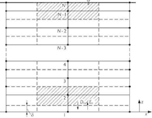
Figure 7.4
Control volumes near bed and water surfaces.
which has the following analytical solution:
a
2
e
−
z
ω
sk
/ε
s
c
k
=
a
1
+
(7.53)
where
a
1
and
a
2
are two constants determined by applying conditions:
c
k
=
c
2
k
at
z
(interface). Inserting Eq. (7.53) with
the obtained
a
1
and
a
2
into Eq. (7.45) yields the following relation for the near-bed
concentration
c
bk
:
=
z
2
(point 2) and
c
k
=
c
bk
at
z
=
z
b
+
δ
e
−
(
z
2
−
z
b
−
δ)ω
sk
/ε
s
c
bk
=
c
2
k
+
c
b
∗
k
[
1
−
]
(7.54)
If
z
2
−
z
b
−
δ
is small, Eq. (7.54) may be approximated with the following linear
relation:
z
b
−
δ)
ω
sk
ε
c
bk
=
c
2
k
+
c
b
∗
k
(
z
2
−
(7.55)
s
The bed-load transport equation (7.46) is a 2-D partial differential equation. It is
discretized by integrating over the horizontal 2-D control volume shown in Fig. 4.21
with the values of
q
b
at cell faces given by a first-order or higher-order upwind scheme.
Note that the 2-D control volume is obtained by projecting the 3-D control volume
onto the horizontal plane, as described in Section 7.2.4. The discretized bed-load
transport equation is
q
n
+
1
bk
,
P
u
n
+
1
q
bk
,
P
u
bk
,
P
A
P
b
W
q
n
+
1
b
E
q
n
+
1
b
S
q
n
+
1
b
N
q
n
+
1
bk
,
N
bk
,
P
−
=
bk
,
W
+
bk
,
E
+
bk
,
S
+
t
b
P
q
n
+
1
−
bk
,
P
+
S
bk
,
P
(7.56)