Mathematical description of flow and sediment transport - Computational River Dynamics - page 15

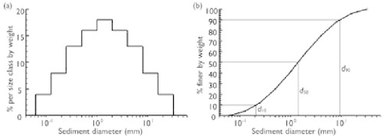
Figure 2.1 Size distribution: (a) histogram and (b) cumulative frequency curve.

shown in Fig. 2.1(a).The cumulative size frequency curve shows the percent of mate-
rial finer than a given sediment size in the total sample, as shown in Fig. 2.1(b). For a
sediment mixture with a normal size distribution, the cumulative size frequency curve
is a straight line on the normal probability paper.

Characteristic diameters
The median diameter, d 50 , is the particle size at which 50% by weight of the sample
is finer. Likewise, d 10 and d 90 are the particle sizes at which 10% and 90% by weight
of the sample are finer, respectively. The diameters d 10 , d 50 , and d 90 can be read from
the cumulative size frequency curve, as shown in Fig. 2.1(b).
The arithmetic mean diameter is determined by

N

d m = p k d k /

100 (2.10)

k = 1

where p k is by percent, and N is the total number of size classes.
The geometric mean diameter is given by

d p 1 / 100
1

d p 2 / 100
2

d p N / 100
N

d g = · · ... · (2.11)

Uniformity
The uniformity of a sediment mixture can be described by the standard deviation:

d 84.1
d 15.9

1 / 2

σ = (2.12)

g

or the gradation coefficient:

d 84.1
d 50 +

1
2

d 50
d 15.9

Gr = (2.13)