2-D numerical models - Computational River Dynamics - page 249

where a P = l = W , E , S , N a p

p P − p P ) F e − F w +

+ A P /( g t ) , S p =− ( A P /( g t ) − (

l

F n − , and F w and F s are the fluxes determined using Eqs. (6.24) and (6.25) in

terms of the approximate velocities U i , w abd U i , s .

F s )

Implementation of boundary conditions

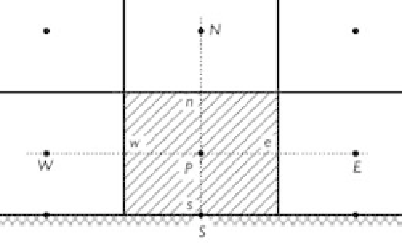
Near a rigid wall, the control volume is shown in Fig. 6.2. The velocity at point S ,
which is located on the wall, is non-slip and has a value of zero. When the x -momentum
equation is integrated over this control volume, as demonstrated in Eq. (4.130), the
convection flux should be zero and the shear stress

xy is determined using Eq. (6.12)
at face s . This shear stress is moved into the source term, thus yielding a zero coefficient
a u x S in Eq. (6.22).
When the y -momentum equation is integrated over the control volume in Fig. 6.2,
the convection flux and the normal stress

τ

τ yy at face s should be zero. Thus, the

coefficient a u y
S

in Eq. (6.22) is zero as well.

Figure 6.2 Control volume near rigid wall.

Because the flux F s is zero, the pressure correction at face s is not needed and,
naturally, a p

S in Eq. (6.28) becomes zero. The pressure (water level) at the boundary
point S can be extrapolated from the values at adjacent internal points.
As mentioned in Section 6.1.2, there are two approaches for handling k and

ε at

the wall boundary. One approach directly specifies the values of k and at center

P in Fig. 6.2, according to Eq. (6.15). The other approach solves the k equation at
the control volume near the wall. When the k equation is integrated over this control
volume, the convection flux at face s and the coefficient a S are set to zero, but the
turbulence generation and dissipation rates at center P are given by Eq. (6.16).
At the inlet, the control volume is shown in Fig. 6.3(a), with face w being on the
inflow side. For the specified total flow discharge Q , Eq. (6.17) cannot directly give
a unique value for the inflow flux at each cell, due to the fact that the flow depth is
also unknown. Iteration is usually needed. At first, a pressure is assumed at face w so
that the inflow velocity and flux can be uniquely obtained using Eq. (6.17). Because
the inflow flux is thereby obtained, the flux correction at face w is zero, and thus the
pressure correction equation becomes

ε

a p a p a p a p

P p P = E p E + S p S + N p N +

S p (6.29)