Geoscience Reference
In-Depth Information
and
P
b
stems from significant vertical velocity gradients near the bottom of the water
body. These terms are related to the bed shear velocity by
P
kb
ε
c
−
1
/
2
f
U
3
=
∗
/
h
and
2
c
1
/
2
c
−
3
/
4
f
U
4
h
2
. The standard values of coefficients
c
P
=
c
c
∗
/
,
c
1
,
c
2
,
σ
k
, and
ε
ε
ε
µ
µ
ε
ε
b
σ
ε
are listed in Table 2.3, while the coefficient
c
is given 3.6 for experimental cases
ε
and 1.8 for field cases (Rodi, 1993).
In analogy to Rastogi and Rodi's depth-averaged standard
k
-
ε
turbulence model,
Wu
et al
. (2004b) adopted the concepts in the non-equilibrium
k
-
ε
turbulence model
of Chen and Kim (1987) and the RNG
k
-
turbulence model of Yakhot
et al
. (1992) in
the depth-averaged 2-D simulation of shallow water flows. The
k
and
ε
ε
equations are
the same as Eqs. (6.10) and (6.11), with coefficients
c
,
c
1
,
c
2
,
σ
k
, and
σ
ε
re-evaluated
µ
ε
ε
according to Table 2.3.
A comparison conducted by Wu
et al
. (2004b) shows that all five depth-averaged
turbulence models described above can give reliable predictions for simple flows, but
for complex flows, the three
k
-
turbulence models generally provide more accurate
results than the two zero-equation turbulence models. Among the three
k
-
ε
turbulence
models, the non-equilibrium and RNG versions perform somewhat better than the
standard version for recirculation flows.
ε
6.1.2 Boundary conditions
Rigid wall boundary conditions
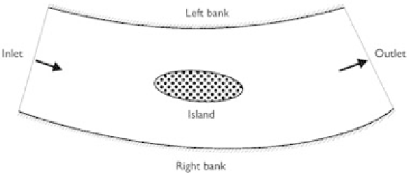
Near a rigid wall, which may be a bank or island as shown in Fig. 6.1, the flow is
quite complex. A very thin viscous sublayer exists near a smooth wall, while roughness
elements on a rough wall affect the flow significantly. Because the velocity gradient
is quite high there, it is of high cost to resolve the flows in the viscous sublayer and
around individual roughness elements. A wall-function approach is often used instead.
The first grid point or cell center (denoted as
P
) adjacent to the wall is placed outside
the viscous sublayer and above the roughness elements, and the resultant wall shear
stress
→
τ
w
is related to the flow velocity
U
P
at point
P
by
w
U
P
→
τ
=−
λ
(6.12)
w
Figure 6.1
A typical horizontal 2-D computational domain.